Urban spatial structure: cities comparison

In this notebook we show the comparison of all the analyzed cities.

Specifically we start by loading the users statistics and figures on stops and pois and we later focus on spatial structure.

Note on data

The data used in this notebook have been provided by Quadrant within the Resilient Urban Planning Analysis Using Smartphone Location Data project of the The World Bank / Global Facility for Disaster Reduction and Recovery (GFDRR) - contract number 7204724.

Quadrant (An Appen Company) is a global leader in mobile location data, POI data, and corresponding compliance services. Quadrant provides anonymised location data and location-based business solutions that are fit for purpose, authentic, easy to use, and simple to organise. We offer data for almost all countries in the world, with hundreds of millions of unique devices and tens of billions of events per month, allowing our clients to perform location analyses, derive location-based intelligence, and make well-informed business decisions. Our data is gathered directly from first party opt-in mobile devices through a server-to-server integration with trusted publisher partners, delivering genuine and reliable raw GPS data unlike other location data sources relying heavily on Bidstream. Our consent management platform, QCMP, ensures that our data is compliant with applicable consent and opt-out provisions of data privacy laws governing the collection and use of location data.

[1]:

%matplotlib inline
import pandas as pd
import numpy as np
import geopandas as gpd
import matplotlib.pyplot as plt
from datetime import datetime
import sys
import os
from shutil import rmtree
from dask.distributed import Client
from dask import dataframe as dd
import dask
import seaborn as sns
import statsmodels.api as sm
import pytz
import psutil
import multiprocessing
sns.set_context('notebook', font_scale=1.5)

dask.__version__

[1]:

'2022.04.1'

We also import mobilkit as mk to gain access to all the librarie’s capabilities. We import some constant names of columns from the dask_schemas submodule as they will be useful later on.

[2]:

import mobilkit as mk
from mobilkit.spatial import haversine_pairwise
from mobilkit.dask_schemas import (latColName, lonColName,
                                   uidColName, zidColName,
                                   accColName, utcColName,
                                   dttColName, durColName,
                                   locColName, ldtColName,
                                   medLatColName, medLonColName)
from mobilkit.viz import compareLinePlot

Configuration

We start defining the cities to be loaded, where the data are and some auxiliary information for each city.

[3]:

ROOT_IN_FOLDER = '/mnt/data/resilience_analyses'
OUT_FOLDER = '/mnt/data/resilience_analyses/comparison'

DATA_CITIES = {}

[4]:

DATA_CITIES['mumbai'] = {
    'name': 'Mumbai',
    'population': 25632800,
    'aoi_radius_km': 60,
    'to_do': True,
}

DATA_CITIES['ankara'] = {
    'name': 'Ankara',
    'population': 5841050,
    'aoi_radius_km': 30,
    'to_do': True,
}

DATA_CITIES['riyadh'] = {
    'name': 'Riyadh',
    'population': 6623460,
    'aoi_radius_km': 40,
    'to_do': True,
}

DATA_CITIES['rio_de_janeiro'] = {
    'name': 'Rio de Janeiro',
    'population': 12545800,
    'aoi_radius_km': 50,
    'to_do': True,
}

DATA_CITIES['doha'] = {
    'name': 'Doha',
    'population': 2409370,
    'aoi_radius_km': 35,
    'to_do': True,
}

DATA_CITIES['dhaka'] = {
    'name': 'Dhaka',
    'population': 32033100,
    'aoi_radius_km': 40,
    'to_do': False,
}

DATA_CITIES['bogota'] = {
    'name': 'Bogota',
    'population': 10056200,
    'aoi_radius_km': 30,
    'to_do': False,
}

DATA_CITIES['buenos_aires'] = {
    'name': 'Buenos Aires',
    'population': 16877600,
    'aoi_radius_km': 50,
    'to_do': False,
}

DATA_CITIES['ho_chi_minh'] = {
    'name': 'Ho Chi Minh',
    'population': 16431400,
    'aoi_radius_km': 45,
    'to_do': False,
}

DATA_CITIES['johannesburg'] = {
    'name': 'Johannesburg',
    'population': 13609300,
    'aoi_radius_km': 45,
    'to_do': False,
}

[5]:

os.makedirs(OUT_FOLDER, exist_ok=True)

[ ]:

Create Dask client

Here we create and connect to a dask client. We just specify where we want Dask to store tmp files (the tmp_dask_dir) and the memory limit per worker.

[6]:

tmp_dask_dir = '/mnt/dask_workplace/'
dask.config.set({'temporary_directory': tmp_dask_dir})
os.environ["DASK_TEMPORARY_DIRECTORY"] = tmp_dask_dir

[7]:

n_proc = int(multiprocessing.cpu_count() / 2) - 1
mem_per_proc = psutil.virtual_memory().total * 1.3 / 1e9 / n_proc
client = Client(
    memory_limit='%.01fG'%mem_per_proc,
    n_workers=n_proc,
    threads_per_worker=2
               )
client

2022-05-18 10:23:50,377 - distributed.diskutils - INFO - Found stale lock file and directory '/mnt/dask_workplace/dask-worker-space/worker-p24zfk__', purging

[7]:

Client

Client-d81322a9-d683-11ec-8cfd-4fcacadb0ef4

Connection method: Cluster object	Cluster type: distributed.LocalCluster
Dashboard: http://127.0.0.1:8787/status

Cluster Info

LocalCluster

8a4324b4

Dashboard: http://127.0.0.1:8787/status	Workers: 23
Total threads: 46	Total memory: 162.80 GiB
Status: running	Using processes: True

Scheduler Info

Scheduler

Scheduler-086b2d90-a4ed-4ec6-98f1-c43eca4d1eb0

Comm: tcp://127.0.0.1:39577	Workers: 23
Dashboard: http://127.0.0.1:8787/status	Total threads: 46
Started: Just now	Total memory: 162.80 GiB

Workers

Worker: 0

Comm: tcp://127.0.0.1:43413	Total threads: 2
Dashboard: http://127.0.0.1:34879/status	Memory: 7.08 GiB
Nanny: tcp://127.0.0.1:34595
Local directory: /mnt/dask_workplace/dask-worker-space/worker-g06l_5jx

Worker: 1

Comm: tcp://127.0.0.1:37955	Total threads: 2
Dashboard: http://127.0.0.1:33509/status	Memory: 7.08 GiB
Nanny: tcp://127.0.0.1:45115
Local directory: /mnt/dask_workplace/dask-worker-space/worker-z_yphp7h

Worker: 2

Comm: tcp://127.0.0.1:33719	Total threads: 2
Dashboard: http://127.0.0.1:39179/status	Memory: 7.08 GiB
Nanny: tcp://127.0.0.1:45817
Local directory: /mnt/dask_workplace/dask-worker-space/worker-j98f9cr6

Worker: 3

Comm: tcp://127.0.0.1:42443	Total threads: 2
Dashboard: http://127.0.0.1:45993/status	Memory: 7.08 GiB
Nanny: tcp://127.0.0.1:33181
Local directory: /mnt/dask_workplace/dask-worker-space/worker-hjw0u9nu

Worker: 4

Comm: tcp://127.0.0.1:35249	Total threads: 2
Dashboard: http://127.0.0.1:43719/status	Memory: 7.08 GiB
Nanny: tcp://127.0.0.1:41575
Local directory: /mnt/dask_workplace/dask-worker-space/worker-tltiot4n

Worker: 5

Comm: tcp://127.0.0.1:45519	Total threads: 2
Dashboard: http://127.0.0.1:34813/status	Memory: 7.08 GiB
Nanny: tcp://127.0.0.1:44541
Local directory: /mnt/dask_workplace/dask-worker-space/worker-iitwa8yv

Worker: 6

Comm: tcp://127.0.0.1:36847	Total threads: 2
Dashboard: http://127.0.0.1:43843/status	Memory: 7.08 GiB
Nanny: tcp://127.0.0.1:37263
Local directory: /mnt/dask_workplace/dask-worker-space/worker-l3kryon7

Worker: 7

Comm: tcp://127.0.0.1:42717	Total threads: 2
Dashboard: http://127.0.0.1:39919/status	Memory: 7.08 GiB
Nanny: tcp://127.0.0.1:33989
Local directory: /mnt/dask_workplace/dask-worker-space/worker-4a5scbru

Worker: 8

Comm: tcp://127.0.0.1:46307	Total threads: 2
Dashboard: http://127.0.0.1:41257/status	Memory: 7.08 GiB
Nanny: tcp://127.0.0.1:44345
Local directory: /mnt/dask_workplace/dask-worker-space/worker-nk9yp55r

Worker: 9

Comm: tcp://127.0.0.1:37809	Total threads: 2
Dashboard: http://127.0.0.1:36845/status	Memory: 7.08 GiB
Nanny: tcp://127.0.0.1:44769
Local directory: /mnt/dask_workplace/dask-worker-space/worker-icja90s8

Worker: 10

Comm: tcp://127.0.0.1:41383	Total threads: 2
Dashboard: http://127.0.0.1:34029/status	Memory: 7.08 GiB
Nanny: tcp://127.0.0.1:34227
Local directory: /mnt/dask_workplace/dask-worker-space/worker-f1_hbdlu

Worker: 11

Comm: tcp://127.0.0.1:45327	Total threads: 2
Dashboard: http://127.0.0.1:38431/status	Memory: 7.08 GiB
Nanny: tcp://127.0.0.1:36067
Local directory: /mnt/dask_workplace/dask-worker-space/worker-7r_1ib08

Worker: 12

Comm: tcp://127.0.0.1:39347	Total threads: 2
Dashboard: http://127.0.0.1:33093/status	Memory: 7.08 GiB
Nanny: tcp://127.0.0.1:42525
Local directory: /mnt/dask_workplace/dask-worker-space/worker-3nrswfa4

Worker: 13

Comm: tcp://127.0.0.1:46697	Total threads: 2
Dashboard: http://127.0.0.1:39163/status	Memory: 7.08 GiB
Nanny: tcp://127.0.0.1:44241
Local directory: /mnt/dask_workplace/dask-worker-space/worker-8qwdw6pk

Worker: 14

Comm: tcp://127.0.0.1:33851	Total threads: 2
Dashboard: http://127.0.0.1:35481/status	Memory: 7.08 GiB
Nanny: tcp://127.0.0.1:34973
Local directory: /mnt/dask_workplace/dask-worker-space/worker-qbi_p5bh

Worker: 15

Comm: tcp://127.0.0.1:36233	Total threads: 2
Dashboard: http://127.0.0.1:34953/status	Memory: 7.08 GiB
Nanny: tcp://127.0.0.1:46487
Local directory: /mnt/dask_workplace/dask-worker-space/worker-z5mq1_cq

Worker: 16

Comm: tcp://127.0.0.1:42053	Total threads: 2
Dashboard: http://127.0.0.1:37257/status	Memory: 7.08 GiB
Nanny: tcp://127.0.0.1:33229
Local directory: /mnt/dask_workplace/dask-worker-space/worker-_ijdyjmy

Worker: 17

Comm: tcp://127.0.0.1:36601	Total threads: 2
Dashboard: http://127.0.0.1:38731/status	Memory: 7.08 GiB
Nanny: tcp://127.0.0.1:42787
Local directory: /mnt/dask_workplace/dask-worker-space/worker-pwqdmzuh

Worker: 18

Comm: tcp://127.0.0.1:33239	Total threads: 2
Dashboard: http://127.0.0.1:44239/status	Memory: 7.08 GiB
Nanny: tcp://127.0.0.1:46209
Local directory: /mnt/dask_workplace/dask-worker-space/worker-2bwp1xer

Worker: 19

Comm: tcp://127.0.0.1:38189	Total threads: 2
Dashboard: http://127.0.0.1:34439/status	Memory: 7.08 GiB
Nanny: tcp://127.0.0.1:41665
Local directory: /mnt/dask_workplace/dask-worker-space/worker-vamoa_pb

Worker: 20

Comm: tcp://127.0.0.1:35519	Total threads: 2
Dashboard: http://127.0.0.1:46323/status	Memory: 7.08 GiB
Nanny: tcp://127.0.0.1:43521
Local directory: /mnt/dask_workplace/dask-worker-space/worker-q_i2k9ol

Worker: 21

Comm: tcp://127.0.0.1:33187	Total threads: 2
Dashboard: http://127.0.0.1:39195/status	Memory: 7.08 GiB
Nanny: tcp://127.0.0.1:43115
Local directory: /mnt/dask_workplace/dask-worker-space/worker-l0q87ifp

Worker: 22

Comm: tcp://127.0.0.1:36885	Total threads: 2
Dashboard: http://127.0.0.1:42149/status	Memory: 7.08 GiB
Nanny: tcp://127.0.0.1:43137
Local directory: /mnt/dask_workplace/dask-worker-space/worker-okdzillh

Load the needed data

[8]:

for city, data in DATA_CITIES.items():
    print(data['name'])
    path_users_stats = os.path.join(ROOT_IN_FOLDER, city, 'users_stats.pkl')
    data['users_stats_df'] = pd.read_pickle(path_users_stats)



    path_users_stop_locs = os.path.join(ROOT_IN_FOLDER, city, 'users_stop_locs_df')
    users_stop_locs_df = dd.read_parquet(path_users_stop_locs)
    n_locs = users_stop_locs_df.shape[0].compute()
    data['number_of_locations'] = n_locs

    path_user_locs_stats_hw_separated = os.path.join(ROOT_IN_FOLDER, city,
                                                     'user_locs_stats_hw_separated.pkl')
    data['user_locs_stats_hw_separated'] = pd.read_pickle(path_user_locs_stats_hw_separated)

    path_df_hw_locs_pd = os.path.join(ROOT_IN_FOLDER, city,
                                      'df_hw_locs_pd.pkl')
    data['df_hw_locs_pd'] = pd.read_pickle(path_df_hw_locs_pd)


    data['user_stats_table_df'] = pd.read_pickle(os.path.join(ROOT_IN_FOLDER, city,
                                                      'user_stats_table_df.pkl'))
    data['cleaned_user_stats_table_df'] = pd.read_pickle(os.path.join(ROOT_IN_FOLDER, city,
                                                              'cleaned_user_stats_table_df.pkl'))

    data['out_df_hw_locs'] = pd.read_pickle(os.path.join(ROOT_IN_FOLDER, city, 'out_df_hw_locs.pkl'))
    data['df_cnt_hw_locs'] = pd.read_pickle(os.path.join(ROOT_IN_FOLDER, city, 'out_df_cnt_hw_locs.pkl'))


    data['gdf'] = gpd.read_file(os.path.join(ROOT_IN_FOLDER, city,
                                             'gdf_landuse_rog.gpkg'))

Mumbai
Ankara
Riyadh
Rio de Janeiro
Doha
Dhaka
Bogota
Buenos Aires
Ho Chi Minh
Johannesburg

[9]:

for city, data in  DATA_CITIES.items():
    tmp_stats = data['users_stats_df']
    tot_pings = tmp_stats['pings'].sum()
    avg_pings_per_user_per_day = np.mean([v for pp in tmp_stats['pingsPerDay'].values for v in pp])
    n_days = (tmp_stats['max_day'].max() - tmp_stats['min_day'].min()).days
    avg_pings_per_day = tot_pings / n_days
    data['avg_pings_per_day'] = avg_pings_per_day
    data['avg_pings_per_user_per_day'] = avg_pings_per_user_per_day

    print(city, avg_pings_per_day, avg_pings_per_user_per_day)

mumbai 3346701.6 6.592426995706759
ankara 1020145.9333333333 8.223536963944412
riyadh 2967286.466666667 8.364091005227968
rio_de_janeiro 1758042.0 11.443970860967202
doha 374636.1 5.211704756022236
dhaka 526990.8 4.819173879804474
bogota 2400355.9032258065 11.383109358480972
buenos_aires 5114443.354838709 9.892531696796421
ho_chi_minh 5200092.433333334 15.6421293813728
johannesburg 431136.8 3.4879473430436314

Check representativeness with statistical requirements

We sort the cities by the ratio of the observed monhly users over the city’s population. We check how this ratio decreases as we increase the minimum number of required pings.

[10]:

df_mau = []
for city, data in DATA_CITIES.items():
    tmp_stats = data['users_stats_df']

    for thres in [0,10,20,50,100]:
        tmp_df = tmp_stats.query('pings>=@thres')
        tmp_n = tmp_df.shape[0]
        tmp_p = tmp_df['pings'].sum()

        df_mau.append([data['name'], thres, tmp_n, tmp_p,
                       tmp_n / data['population']*100., data['to_do']])
df_mau = pd.DataFrame(df_mau, columns=['City', 'Min pings', 'N users', 'N pings', 'MAU % pop.', 'Good data'])
df_mau.head(0)

[10]:

	City	Min pings	N users	N pings	MAU % pop.	Good data

[11]:

city_order = sorted(list(df_mau['City'].unique()))

[12]:

g = sns.lineplot(x='Min pings',
                 y='MAU % pop.',
                 hue='City',
                 hue_order=city_order,
                 # style='Good data',
                 # style_order=[True,False],
                 data=df_mau,
            )
plt.semilogy()
plt.title('MAU by minimum raw pings')

# Put the legend out of the figure
g.legend(loc='center left',
         title='City',
         bbox_to_anchor=(1, 0.5))
plt.savefig(os.path.join(OUT_FOLDER, 'mau_users_min_pings.pdf'), bbox_inches='tight')

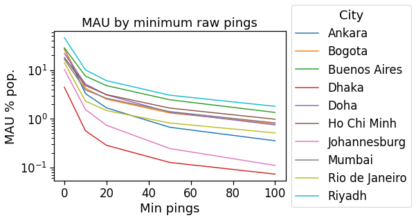
../_images/examples_USS02_CityComparison_18_0.png

[13]:

df_mau[df_mau['Min pings']==10][['City','MAU % pop.']]

[13]:

	City	MAU % pop.
1	Mumbai	3.903885
6	Ankara	3.279650
11	Riyadh	10.101880
16	Rio de Janeiro	2.299128
21	Doha	5.172929
26	Dhaka	0.566093
31	Bogota	4.214564
36	Buenos Aires	7.519973
41	Ho Chi Minh	4.818226
46	Johannesburg	1.548008

[ ]:

[14]:

df_mau_homeWork = None
for city, data in DATA_CITIES.items():
    tmp_stats = data['df_cnt_hw_locs']
    tmp_min_days = tmp_stats['n_days'].min()

    tmp_df = tmp_stats.query('n_days ==%d & n_hours == 10' % max(tmp_min_days, 4)).copy(deep=True)
    tmp_df['City'] = data['name']
    tmp_df['MAU % pop.'] = tmp_df['n_users'] / data['population'] * 100
    tmp_df['MAU with home % pop.'] = tmp_df['with_home_users'] / data['population'] * 100
    tmp_df['MAU with work % pop.'] = tmp_df['with_work_users'] / data['population'] * 100

    df_mau_homeWork = pd.concat((tmp_df, df_mau_homeWork),
                                sort=True, ignore_index=True)
df_mau_homeWork.head(0)

[14]:

	City	MAU % pop.	MAU with home % pop.	MAU with work % pop.	delta_count	delta_duration	home_work_same_area_users	home_work_same_area_users_frac	n_days	n_hours	n_users	tot_duration	with_home_users	with_work_users

[ ]:

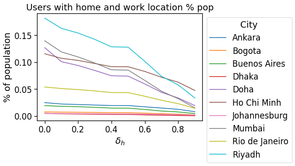
[15]:

fig, ax = plt.subplots(1,1,figsize=(6,4))
sns.lineplot(x='delta_duration', y='MAU % pop.',
             data=df_mau_homeWork,
             hue='City',
             hue_order=city_order,
            )
# plt.semilogy()
plt.legend(loc=2, bbox_to_anchor=[1,1], title='City',)
plt.xlabel(r"$\delta_h$")
plt.ylabel("% of population")
plt.title('Users with home and work location % pop')
fig.savefig(os.path.join(OUT_FOLDER, 'mau_users_with_home_work.pdf'), bbox_inches='tight')

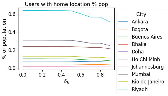
../_images/examples_USS02_CityComparison_23_0.png

[16]:

fig, ax = plt.subplots(1,1,figsize=(6,4))
sns.lineplot(x='delta_duration', y='MAU with home % pop.',
             data=df_mau_homeWork,
             hue='City',
             hue_order=city_order,
            )
# plt.semilogy()
plt.legend(loc=2, bbox_to_anchor=[1,1], title='City',)
plt.xlabel(r"$\delta_h$")
plt.ylabel("% of population")
plt.title('Users with home location % pop')
fig.savefig(os.path.join(OUT_FOLDER, 'mau_users_with_home.pdf'), bbox_inches='tight')

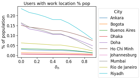
../_images/examples_USS02_CityComparison_24_0.png

[17]:

fig, ax = plt.subplots(1,1,figsize=(6,4))
sns.lineplot(x='delta_duration', y='MAU with work % pop.',
             data=df_mau_homeWork,
             hue='City',
             hue_order=city_order,
            )
# plt.semilogy()
plt.legend(loc=2, bbox_to_anchor=[1,1], title='City',)
plt.xlabel(r"$\delta_h$")
plt.ylabel("% of population")
plt.title('Users with work location % pop')
fig.savefig(os.path.join(OUT_FOLDER, 'mau_users_with_work.pdf'), bbox_inches='tight')

../_images/examples_USS02_CityComparison_25_0.png

Spatial structure

We test the universality of the spatial structure of the cities by comparing the functioning of the different indicators in the different context.

[1]:

min_count_per_area = 10

[19]:

df_spatial_areas = None
for city, data in DATA_CITIES.items():
    if not data['to_do']: continue

    tmp_df = data['gdf'].query('rog_home_count >= @min_count_per_area').copy(deep=True)
    tmp_df['City'] = data['name']
    tmp_df['cbd_dist_norm'] = tmp_df['cbd_dist'] / data['aoi_radius_km']
    tmp_df['cbd_dist_bin_norm'] = np.round(tmp_df['cbd_dist_norm'], decimals=1)

    df_spatial_areas = pd.concat((tmp_df, df_spatial_areas),
                                sort=True, ignore_index=True)
df_spatial_areas.head(0)

[19]:

	City	avg_realD_frac_osmD	avg_realT_frac_osmT	bottom	cbd_dist	cbd_dist_bin	cbd_dist_bin_norm	cbd_dist_norm	cluster	geometry	...	ttd_min	ttd_std	work_home_osrm_dist_avg	work_home_osrm_dist_max	work_home_osrm_dist_min	work_home_osrm_dist_std	work_home_osrm_time_avg	work_home_osrm_time_max	work_home_osrm_time_min	work_home_osrm_time_std

0 rows × 76 columns

[20]:

df_spatial_users = None
for city, data in DATA_CITIES.items():
    if not data['to_do']: continue

    tmp_df = data['cleaned_user_stats_table_df'].copy(deep=True)
    tmp_df['City'] = data['name']

    tmp_df['aoi_radius_km'] = data['aoi_radius_km']

    tmp_df['cbd_dist_norm'] = tmp_df['cbd_dist'] / tmp_df['aoi_radius_km']
    tmp_df['cbd_dist_bin_norm'] = np.round(tmp_df['cbd_dist_norm'], decimals=1)

    tmp_df['closest_cbd_dist_norm'] = tmp_df['closest_cbd_dist'] / tmp_df['aoi_radius_km']
    tmp_df['closest_cbd_dist_bin_norm'] = np.round(tmp_df['closest_cbd_dist_norm'], decimals=1)

    df_spatial_users = pd.concat((tmp_df, df_spatial_users),
                                sort=True, ignore_index=True)
df_spatial_users.head(0)

[20]:

	City	aoi_radius_km	avg	avg_realD_frac_osmD	avg_realT_frac_osmT	cbd_dist	cbd_dist_bin	cbd_dist_bin_norm	cbd_dist_norm	closest_cbd_dist	...	speed_trips_hw	speed_trips_wh	time_trips_hw	time_trips_wh	tot_pings	ttd	work_home_osrm_dist	work_home_osrm_time	work_loc_ID	work_pings

0 rows × 49 columns

[21]:

city_todo_order = sorted(list(df_spatial_areas['City'].unique()))

[22]:

def plotLines(
    x, y, data,
    hue='City',
    hue_order=city_todo_order,
    figsize=(12,5),
    xlabel='ylabel',
    ylabel='xlabel',
    title=None,
    xlim=None,
    ylim=None,
    kwargs_leg={},
    tight=True,
    **kwargs,
):
    fig, ax = plt.subplots(1,1,figsize=figsize)
    g = sns.lineplot(data=data,
                 x=x,
                 y=y,
                 hue=hue,
                 hue_order=hue_order,
                ax=ax,
                 **kwargs
    )
    g.legend(loc=2, bbox_to_anchor=[1,1], title=hue, **kwargs_leg)

    ax.set_title(title)
    ax.set_xlabel(xlabel)
    ax.set_ylabel(ylabel)

    if xlim:
        ax.set_xlim(xlim)
    if ylim:
        ax.set_ylim(ylim)
    if tight:
        fig.tight_layout()
    return fig, ax

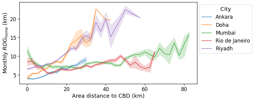
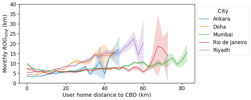
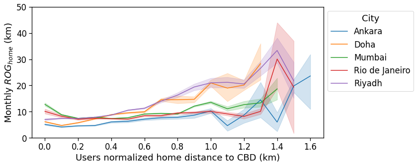
Radius of Gyration (ROG) vs. distance to Central Business District

In this first plot we observe that Doha and Riyadh display a strong monocentric pattern, whereas the other cities feature a non-monotonic increase of the ROG (centered on the users’ homes) as we move away from the CBD.

[23]:

fig, ax = plotLines(
    data=df_spatial_areas,
    x='cbd_dist_bin',
    y='rog_home_mean',
    hue='City',
    hue_order=city_todo_order,
    xlabel=r'Area distance to CBD (km)',
    ylabel=r'Monthly $ROG_{home}$ (km)',
    # title=r'Per area $ROG_{home}$ vs. distance to CBD'
)
fig.savefig(os.path.join(OUT_FOLDER, 'rog_home_month_area_cbd.pdf'), bbox_inches='tight')

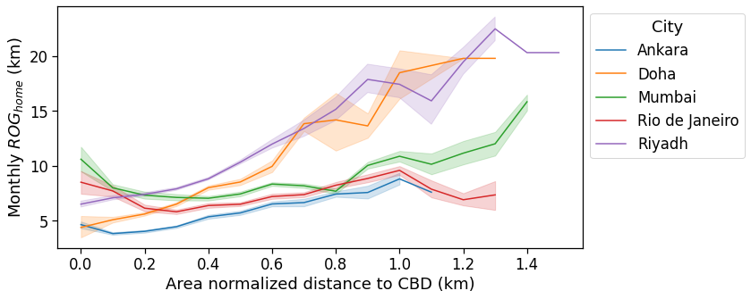
../_images/examples_USS02_CityComparison_33_0.png

The same holds if we normalize the distance from the CBD by the city’s radius.

[24]:

fig, ax = plotLines(
    data=df_spatial_areas,
    x='cbd_dist_bin_norm',
    y='rog_home_mean',
    hue='City',
    hue_order=city_todo_order,
    xlabel=r'Area normalized distance to CBD (km)',
    ylabel=r'Monthly $ROG_{home}$ (km)',
    # title=r'Per area $ROG_{home}$ vs. normalized distance to CBD'
)
fig.savefig(os.path.join(OUT_FOLDER, 'rog_home_month_area_cbd_norm.pdf'), bbox_inches='tight')

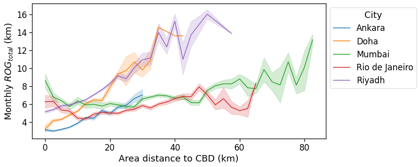
../_images/examples_USS02_CityComparison_35_0.png

The same holds if we measure the ROG with respect to the user’s baricenter.

[25]:

fig, ax = plotLines(
    data=df_spatial_areas,
    x='cbd_dist_bin',
    y='rog_total_mean',
    hue='City',
    hue_order=city_todo_order,
    xlabel=r'Area distance to CBD (km)',
    ylabel=r'Monthly $ROG_{total}$ (km)',
    # title=r'Per area $ROG_{total}$ vs. distance to CBD'
)
fig.savefig(os.path.join(OUT_FOLDER, 'rog_total_month_area_cbd.pdf'), bbox_inches='tight')

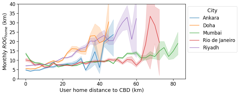
../_images/examples_USS02_CityComparison_37_0.png

[26]:

fig, ax = plotLines(
    data=df_spatial_users,
    x='cbd_dist_bin',
    y='rog_home',
    hue='City',
    hue_order=city_todo_order,
    xlabel=r'User home distance to CBD (km)',
    ylabel=r'Monthly $ROG_{home}$ (km)',
    # title=r'Per user $ROG_{home}$ vs. home distance to CBD',
    ylim=(0,40),
)
fig.savefig(os.path.join(OUT_FOLDER, 'rog_home_month_user_cbd.pdf'), bbox_inches='tight')

../_images/examples_USS02_CityComparison_38_0.png

[27]:

fig, ax = plotLines(
    data=df_spatial_users,
    x='cbd_dist_bin',
    y='rog_total',
    hue='City',
    hue_order=city_todo_order,
    xlabel=r'User home distance to CBD (km)',
    ylabel=r'Monthly $ROG_{total}$ (km)',
    # title=r'Per user $ROG_{total}$ vs. home distance to CBD',
    ylim=(0,40),
)
fig.savefig(os.path.join(OUT_FOLDER, 'rog_total_month_user_cbd.pdf'), bbox_inches='tight')

../_images/examples_USS02_CityComparison_39_0.png

[28]:

fig, ax = plotLines(
    data=df_spatial_users,
    x='cbd_dist_bin_norm',
    y='rog_home',
    hue='City',
    hue_order=city_todo_order,
    xlabel=r'Users normalized home distance to CBD (km)',
    ylabel=r'Monthly $ROG_{home}$ (km)',
    # title=r'Per user $ROG_{home}$ vs. normalized home distance to CBD',
    ylim=(0,50),
)
fig.savefig(os.path.join(OUT_FOLDER, 'rog_home_month_user_cbd_norm.pdf'), bbox_inches='tight')

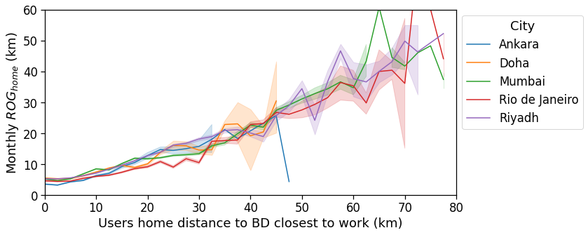
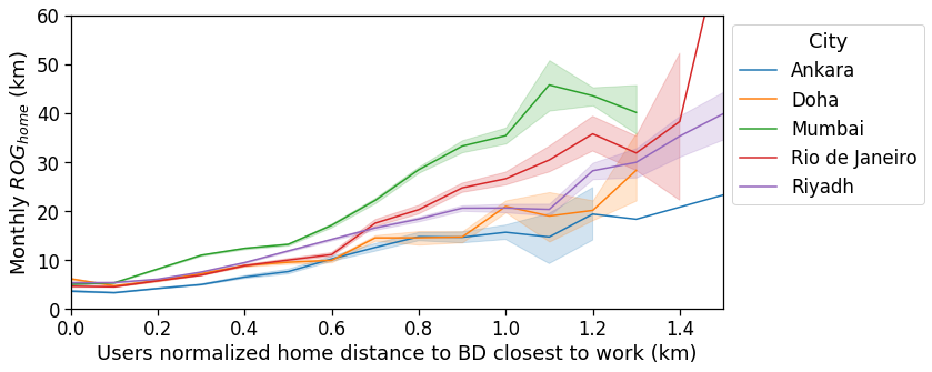
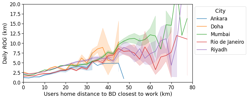
../_images/examples_USS02_CityComparison_40_0.png

Radius of Gyration (ROG) vs. distance to Business District closest to workplace

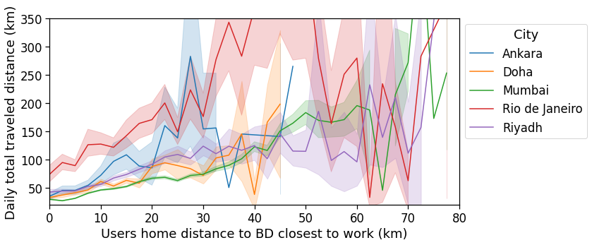
If we instead compte the average ROG for users with the home at a given distance from the BD closest to the user’s workplace, all the cities collapse on a single curve: the new definition of distance from user-dependent BD instead of the unique CBD cancels out the polycentric structure of the city and all the signals lie on a single, monotonically increasing line.

[29]:

fig, ax = plotLines(
    data=df_spatial_users,
    x='closest_cbd_dist_bin',
    y='rog_home',
    hue='City',
    hue_order=city_todo_order,
    xlabel=r'Users home distance to BD closest to work (km)',
    ylabel=r'Monthly $ROG_{home}$ (km)',
    # title=r'Per user $ROG_{home}$ vs. home distance to BD closest to workplace',
    xlim=[0,80],
    ylim=(0,60),
)
fig.savefig(os.path.join(OUT_FOLDER, 'rog_home_month_user_cbd_closest.pdf'), bbox_inches='tight')

../_images/examples_USS02_CityComparison_42_0.png

[30]:

fig, ax = plotLines(
    data=df_spatial_users,
    x='closest_cbd_dist_bin_norm',
    y='rog_home',
    hue='City',
    hue_order=city_todo_order,
    xlabel=r'Users normalized home distance to BD closest to work (km)',
    ylabel=r'Monthly $ROG_{home}$ (km)',
    # title=r'Per user $ROG_{home}$ vs. normalized home distance to BD closest to workplace',
    xlim=[0,1.5],
    ylim=(0,60),
)
fig.savefig(os.path.join(OUT_FOLDER, 'rog_home_month_user_cbd_closest_norm.pdf'), bbox_inches='tight')

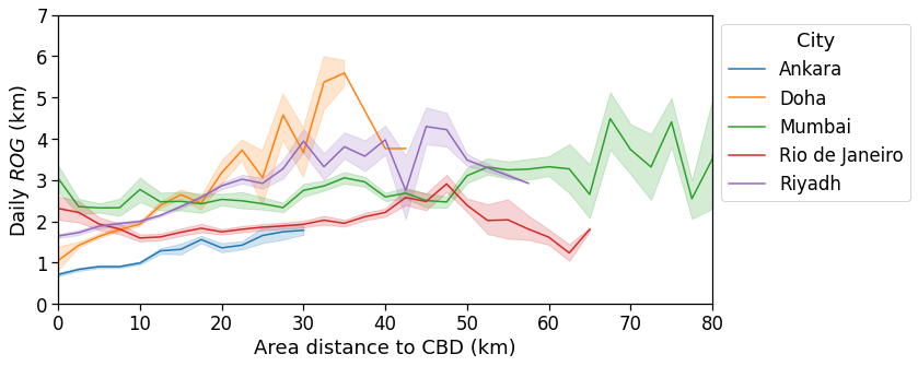
../_images/examples_USS02_CityComparison_43_0.png

Daily Radius of Gyration (ROG) vs. distance to Business District closest to workplace

[31]:

fig, ax = plotLines(
    data=df_spatial_areas,
    x='cbd_dist_bin',
    y='rog_mean',
    hue='City',
    hue_order=city_todo_order,
    xlabel=r'Area distance to CBD (km)',
    ylabel=r'Daily $ROG$ (km)',
    # title=r'Per area $ROG$ vs. distance to CBD',
    xlim=[0,80],
    ylim=(0,7),
)
fig.savefig(os.path.join(OUT_FOLDER, 'rog_daily_area_cbd.pdf'), bbox_inches='tight')

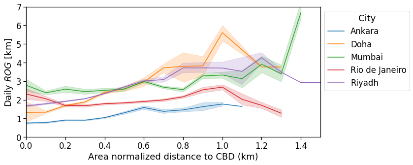
../_images/examples_USS02_CityComparison_45_0.png

[32]:

fig, ax = plotLines(
    data=df_spatial_areas,
    x='cbd_dist_bin_norm',
    y='rog_mean',
    hue='City',
    hue_order=city_todo_order,
    xlabel=r'Area normalized distance to CBD (km)',
    ylabel=r'Daily $ROG$ [km]',
    # title=r'Per area $ROG$ vs. normalized distance to CBD',
    ylim=(0,7),
    xlim=[0,1.5]
)
fig.savefig(os.path.join(OUT_FOLDER, 'rog_daily_area_cbd_norm.pdf'), bbox_inches='tight')

../_images/examples_USS02_CityComparison_46_0.png

[33]:

fig, ax = plotLines(
    data=df_spatial_users,
    x='closest_cbd_dist_bin',
    y='rog',
    hue='City',
    hue_order=city_todo_order,
    xlabel=r'Users home distance to BD closest to work (km)',
    ylabel=r'Daily $ROG$ (km)',
    # title=r'Per user $ROG$ vs. home distance to BD closest to workplace',
    ylim=(0,20),
    xlim=[0,80],
)
fig.savefig(os.path.join(OUT_FOLDER, 'rog_daily_user_cbd_closest.pdf'), bbox_inches='tight')

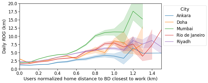
../_images/examples_USS02_CityComparison_47_0.png

[34]:

fig, ax = plotLines(
    data=df_spatial_users,
    x='closest_cbd_dist_bin_norm',
    y='rog',
    hue='City',
    hue_order=city_todo_order,
    xlabel=r'Users normalized home distance to BD closest to work (km)',
    ylabel=r'Daily $ROG$ (km)',
    # title=r'Per user daily $ROG$ vs. normalized home distance to BD closest to workplace',
    xlim=[0,1.5],
    ylim=(0,20),
)
fig.savefig(os.path.join(OUT_FOLDER, 'rog_daily_user_cbd_closest_norm.pdf'), bbox_inches='tight')

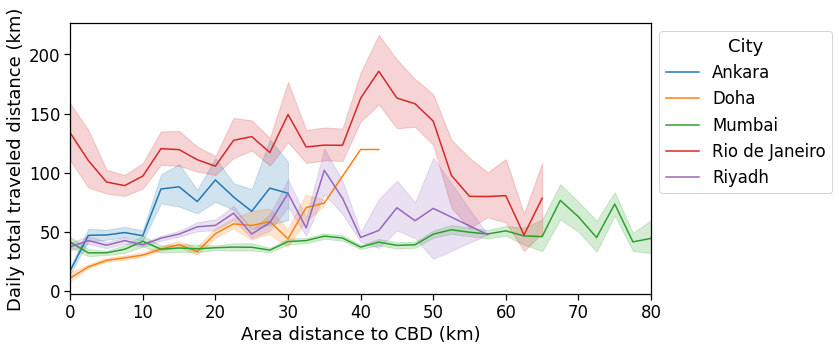
../_images/examples_USS02_CityComparison_48_0.png

Total Traveled Distance (TTD) vs. distance to Central Business District

For this and the next indicators we observe the same behavior. We simply reports all the plots to display the insights gained with the spatial structure analyses of the previous notebook.

[62]:

fig, ax = plotLines(
    data=df_spatial_areas,
    x='cbd_dist_bin',
    y='ttd_mean',
    hue='City',
    hue_order=city_todo_order,
    xlabel=r'Area distance to CBD (km)',
    ylabel='Daily total traveled distance (km)',
    # title=r'Per area daily $TTD$ vs. distance to CBD'
    xlim=[0,80],
)
fig.savefig(os.path.join(OUT_FOLDER, 'ttd_daily_area_cbd.pdf'), bbox_inches='tight')

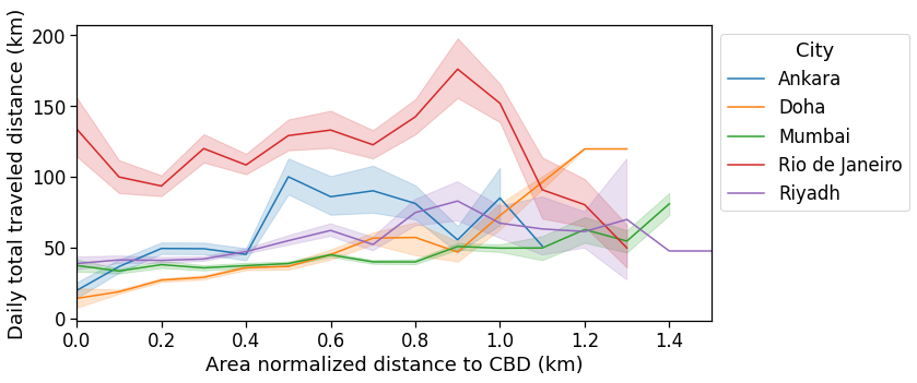
../_images/examples_USS02_CityComparison_50_0.png

[63]:

fig, ax = plotLines(
    data=df_spatial_areas,
    x='cbd_dist_bin_norm',
    y='ttd_mean',
    hue='City',
    hue_order=city_todo_order,
    xlabel=r'Area normalized distance to CBD (km)',
    ylabel=r'Daily total traveled distance (km)',
    # title=r'Per area daily $TTD$ vs. normalized distance to CBD'
    xlim=[0,1.5],
)
fig.savefig(os.path.join(OUT_FOLDER, 'ttd_daily_area_cbd_norm.pdf'), bbox_inches='tight')

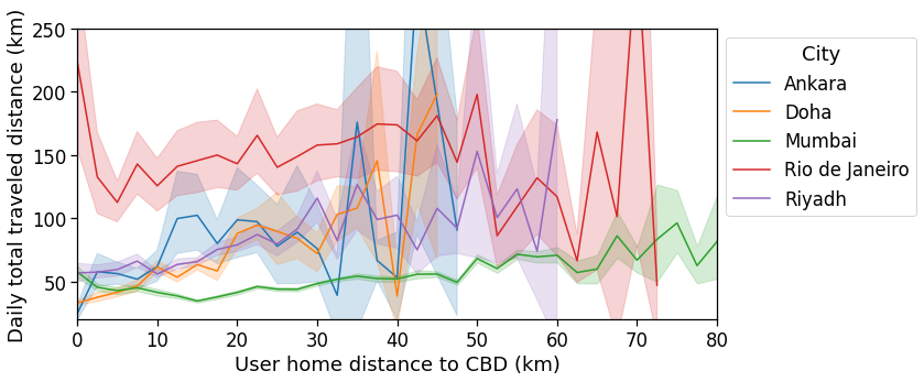
../_images/examples_USS02_CityComparison_51_0.png

[37]:

fig, ax = plotLines(
    data=df_spatial_users,
    x='cbd_dist_bin',
    y='ttd',
    hue='City',
    hue_order=city_todo_order,
    xlabel=r'User home distance to CBD (km)',
    ylabel=r'Daily total traveled distance (km)',
    # title=r'Per user $TTD$ vs. home distance to CBD',
    xlim=[0,80],
    ylim=(20,250),
)
fig.savefig(os.path.join(OUT_FOLDER, 'ttd_daily_user_cbd.pdf'), bbox_inches='tight')

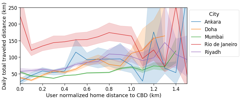
../_images/examples_USS02_CityComparison_52_0.png

[38]:

fig, ax = plotLines(
    data=df_spatial_users,
    x='cbd_dist_bin_norm',
    y='ttd',
    hue='City',
    hue_order=city_todo_order,
    xlabel=r'User normalized home distance to CBD (km)',
    ylabel=r'Daily total traveled distance (km)',
    # title=r'Per user $TTD$ vs. normalized home distance to CBD',
    xlim=[0,1.5],
    ylim=(20,250),
)
fig.savefig(os.path.join(OUT_FOLDER, 'ttd_daily_user_cbd_norm.pdf'), bbox_inches='tight')

../_images/examples_USS02_CityComparison_53_0.png

Total Traveled Distance (TTD) vs. distance to Business District closest to workplace

[39]:

fig, ax = plotLines(
    data=df_spatial_users,
    x='closest_cbd_dist_bin',
    y='ttd',
    hue='City',
    hue_order=city_todo_order,
    xlabel=r'Users home distance to BD closest to work (km)',
    ylabel=r'Daily total traveled distance (km)',
    # title=r'Per user daily $TTD$ vs. home distance to BD closest to workplace',
    xlim=[0,80],
    ylim=(20,350),
)
fig.savefig(os.path.join(OUT_FOLDER, 'ttd_daily_user_cbd_closest.pdf'), bbox_inches='tight')

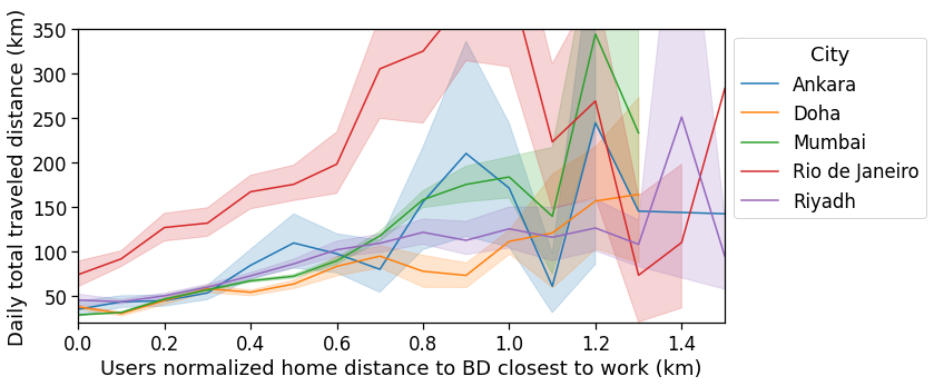
../_images/examples_USS02_CityComparison_55_0.png

[40]:

fig, ax = plotLines(
    data=df_spatial_users,
    x='closest_cbd_dist_bin_norm',
    y='ttd',
    hue='City',
    hue_order=city_todo_order,
    xlabel=r'Users normalized home distance to BD closest to work (km)',
    ylabel=r'Daily total traveled distance (km)',
    # title=r'Per user daily $TTD$ vs. normalized home distance to BD closest to workplace',
    xlim=[0,1.5],
    ylim=(20,350),
)
fig.savefig(os.path.join(OUT_FOLDER, 'ttd_daily_user_cbd_closest_norm.pdf'), bbox_inches='tight')

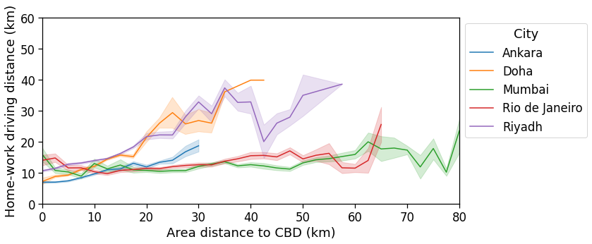
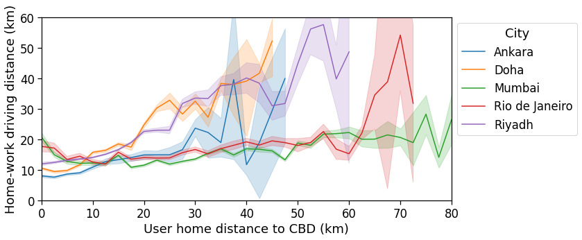
../_images/examples_USS02_CityComparison_56_0.png

Home-work distance vs. distance to Central Business District

[41]:

df_spatial_areas['home_work_osrm_dist_avg_km'] = df_spatial_areas['home_work_osrm_dist_avg'] / 1e3

[42]:

fig, ax = plotLines(
    data=df_spatial_areas,
    x='cbd_dist_bin',
    y='home_work_osrm_dist_avg_km',
    hue='City',
    hue_order=city_todo_order,
    xlabel=r'Area distance to CBD (km)',
    ylabel=r'Home-work driving distance (km)',
    # title=r'Per area $D^{OSRM}_{home,work}$ vs. normalized distance to CBD',
    xlim=[0,80],
    ylim=(0,60),
)
fig.savefig(os.path.join(OUT_FOLDER, 'home_work_dist_area_cbd.pdf'), bbox_inches='tight')

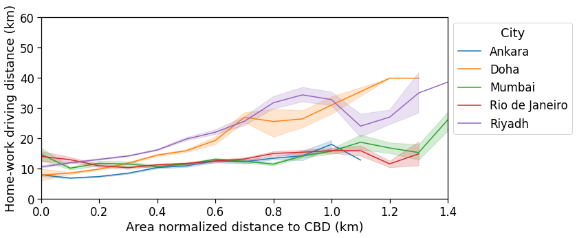
../_images/examples_USS02_CityComparison_59_0.png

[43]:

fig, ax = plotLines(
    data=df_spatial_areas,
    x='cbd_dist_bin_norm',
    y='home_work_osrm_dist_avg_km',
    hue='City',
    hue_order=city_todo_order,
    xlabel=r'Area normalized distance to CBD (km)',
    ylabel=r'Home-work driving distance (km)',
    # title=r'Per area $D^{OSRM}_{home,work}$ vs. normalized distance to CBD',
    xlim=[0,1.4],
    ylim=(0,60),
)
fig.savefig(os.path.join(OUT_FOLDER, 'home_work_dist_area_cbd_norm.pdf'), bbox_inches='tight')

../_images/examples_USS02_CityComparison_60_0.png

[44]:

fig, ax = plotLines(
    data=df_spatial_users,
    x='cbd_dist_bin',
    y='home_work_osrm_dist_km',
    hue='City',
    hue_order=city_todo_order,
    xlabel=r'User home distance to CBD (km)',
    ylabel=r'Home-work driving distance (km)',
    # title=r'Per user $D^{OSRM}_{home,work}$ vs. distance to CBD',
    xlim=[0,80],
    ylim=(0,60),
)
fig.savefig(os.path.join(OUT_FOLDER, 'home_work_dist_user_cbd.pdf'), bbox_inches='tight')

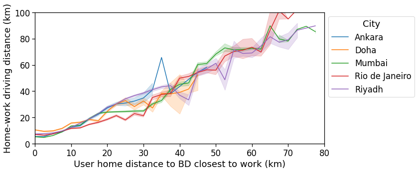
../_images/examples_USS02_CityComparison_61_0.png

Home-work distance vs. distance to Business District closest to homeplace

[45]:

fig, ax = plotLines(
    data=df_spatial_users,
    x='closest_cbd_dist_bin',
    y='home_work_osrm_dist_km',
    hue='City',
    hue_order=city_todo_order,
    xlabel=r'User home distance to BD closest to work (km)',
    ylabel=r'Home-work driving distance (km)',
    # title=r'Per user $D^{OSRM}_{home,work}$ vs. home distance to BD closest to workplace',
    xlim=[0,80],
    ylim=(0,100),
)
fig.savefig(os.path.join(OUT_FOLDER, 'home_work_dist_user_cbd_closest.pdf'), bbox_inches='tight')

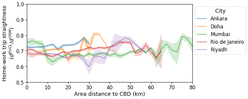
../_images/examples_USS02_CityComparison_63_0.png

Home-work distance ratio (Euclidean/osrm) vs. distance to Central Business District

[46]:

fig, ax = plotLines(
    data=df_spatial_areas,
    x='cbd_dist_bin',
    y='avg_realD_frac_osmD',
    hue='City',
    hue_order=city_todo_order,
    xlabel=r'Area distance to CBD (km)',
    ylabel='Home-work trip straightness\n' + r'$(d^{EUCL} / d^{OSM})$',
    # title=r'Per area home-work $D^{EUCL} / D^{OSRM}$ distance vs. norm. distance to CBD',
    xlim=[0,80],
    ylim=(.5,1.),
)
fig.savefig(os.path.join(OUT_FOLDER, 'home_work_dist_fraction_area_cbd.pdf'), bbox_inches='tight')

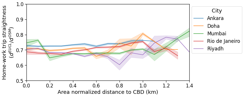
../_images/examples_USS02_CityComparison_65_0.png

[47]:

fig, ax = plotLines(
    data=df_spatial_areas,
    x='cbd_dist_bin_norm',
    y='avg_realD_frac_osmD',
    hue='City',
    hue_order=city_todo_order,
    xlabel=r'Area normalized distance to CBD (km)',
    ylabel='Home-work trip straightness\n' + r'$(d^{EUCL} / d^{OSM})$',
    # title=r'Per area home-work $D^{EUCL} / D^{OSRM}$ distance vs. norm. distance to CBD',
    xlim=[0,1.4],
    ylim=(.5,1.),
)
fig.savefig(os.path.join(OUT_FOLDER, 'home_work_dist_fraction_area_cbd_norm.pdf'), bbox_inches='tight')

../_images/examples_USS02_CityComparison_66_0.png

[48]:

fig, ax = plotLines(
    data=df_spatial_users,
    x='cbd_dist_bin',
    y='avg_realD_frac_osmD',
    hue='City',
    hue_order=city_todo_order,
    xlabel=r'User home distance to CBD (km)',
    ylabel='Home-work trip straightness\n' + r'$(d^{EUCL} / d^{OSM})$',
    # title=r'Per user home-work $D^{EUCL} / D^{OSRM}$ distance vs. home distance to CBD',
    xlim=[0,80],
    ylim=(.5,1.),
)
fig.savefig(os.path.join(OUT_FOLDER, 'home_work_dist_fraction_user_cbd.pdf'), bbox_inches='tight')

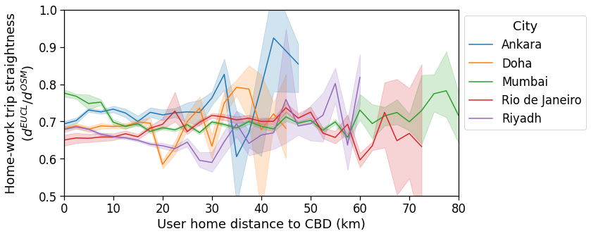
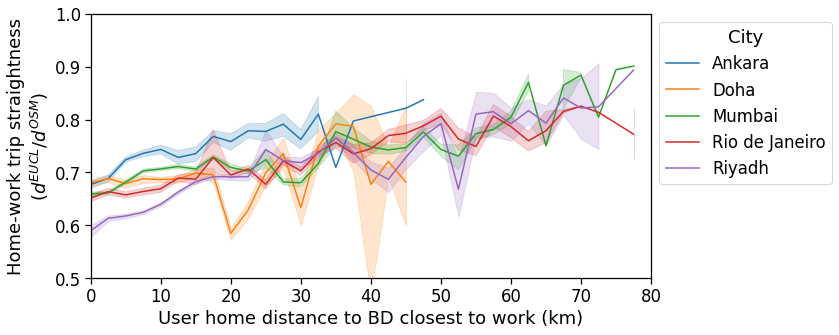
../_images/examples_USS02_CityComparison_67_0.png

Home-work distance ratio (Euclidean/osrm) vs. distance to Business District closest to workplace

[49]:

fig, ax = plotLines(
    data=df_spatial_users,
    x='closest_cbd_dist_bin',
    y='avg_realD_frac_osmD',
    hue='City',
    hue_order=city_todo_order,
    xlabel=r'User home distance to BD closest to work (km)',
    ylabel='Home-work trip straightness\n' + r'$(d^{EUCL} / d^{OSM})$',
    # title=r'Per user home-work $D^{EUCL} / D^{OSRM}$ dist. vs. home dist. to BD closest to work',
    xlim=(0,80),
    ylim=(.5,1),
)
fig.savefig(os.path.join(OUT_FOLDER, 'home_work_dist_fraction_user_cbd_closest.pdf'), bbox_inches='tight')

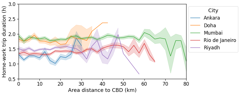
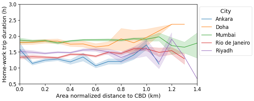
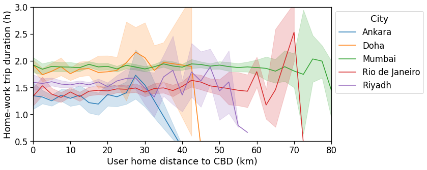
../_images/examples_USS02_CityComparison_69_0.png

Home-work duration vs. distance to Central Business District

[50]:

fig, ax = plotLines(
    data=df_spatial_areas,
    x='cbd_dist_bin',
    y='time_trips_hw_avg',
    hue='City',
    hue_order=city_todo_order,
    xlabel=r'Area distance to CBD (km)',
    ylabel='Home-work trip duration (h)',
    # title=r'Per area home-work $t^{REAL}$ duration vs. norm. distance to CBD',
    xlim=(0,80),
    ylim=(.5,3),
)
fig.savefig(os.path.join(OUT_FOLDER, 'home_work_duration_real_area_cbd.pdf'), bbox_inches='tight')

../_images/examples_USS02_CityComparison_71_0.png

[51]:

fig, ax = plotLines(
    data=df_spatial_areas,
    x='cbd_dist_bin_norm',
    y='time_trips_hw_avg',
    hue='City',
    hue_order=city_todo_order,
    xlabel=r'Area normalized distance to CBD (km)',
    ylabel='Home-work trip duration (h)',
    # title=r'Per area home-work $t^{REAL}$ duration vs. norm. distance to CBD',
    xlim=(0,1.4),
    ylim=(.5,3),
)
fig.savefig(os.path.join(OUT_FOLDER, 'home_work_duration_real_area_cbd_norm.pdf'), bbox_inches='tight')

../_images/examples_USS02_CityComparison_72_0.png

[52]:

fig, ax = plotLines(
    data=df_spatial_users,
    x='cbd_dist_bin',
    y='time_trips_hw',
    hue='City',
    hue_order=city_todo_order,
    xlabel=r'User home distance to CBD (km)',
    ylabel='Home-work trip duration (h)',
    # title=r'Per user home-work $t^{REAL}$ duration vs. home distance to CBD',
    xlim=(0,80),
    ylim=(.5,3),
)
fig.savefig(os.path.join(OUT_FOLDER, 'home_work_duration_real_user_cbd.pdf'), bbox_inches='tight')

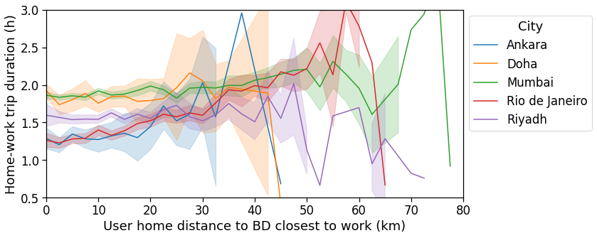
../_images/examples_USS02_CityComparison_73_0.png

Home-work duration vs. distance to Business District closest to workplace

[53]:

fig, ax = plotLines(
    data=df_spatial_users,
    x='closest_cbd_dist_bin',
    y='time_trips_hw',
    hue='City',
    hue_order=city_todo_order,
    xlabel=r'User home distance to BD closest to work (km)',
    ylabel='Home-work trip duration (h)',
    #  title=r'Per user home-work $t^{REAL}$ duration vs. home dist. to BD closest to workplace',
    xlim=(0,80),
    ylim=(.5,3),
)
fig.savefig(os.path.join(OUT_FOLDER, 'home_work_duration_real_user_cbd_closest.pdf'), bbox_inches='tight')

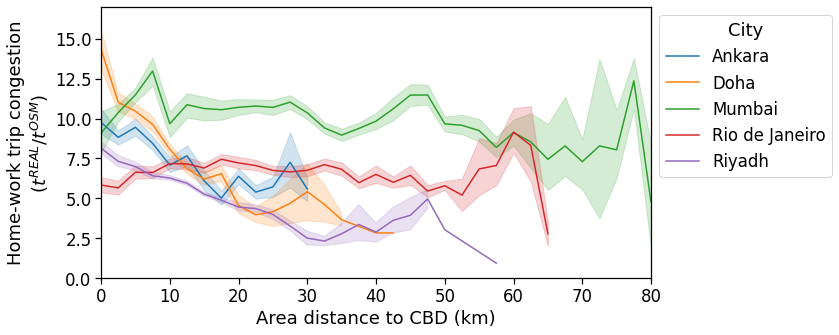
../_images/examples_USS02_CityComparison_75_0.png

Home-work duration ratio (real/osrm) vs. distance to Central Business District

[54]:

fig, ax = plotLines(
    data=df_spatial_areas,
    x='cbd_dist_bin',
    y='avg_realT_frac_osmT',
    hue='City',
    hue_order=city_todo_order,
    xlabel=r'Area distance to CBD (km)',
    ylabel='Home-work trip congestion\n' + r'($t^{REAL} / t^{OSM}$)',
    # title=r'Per area home-work $t^{REAL} / t^{OSRM}$ duration vs. norm. distance to CBD',
    xlim=(0,80),
    ylim=(0,17),
)
fig.savefig(os.path.join(OUT_FOLDER, 'home_work_duration_fraction_area_cbd.pdf'), bbox_inches='tight')

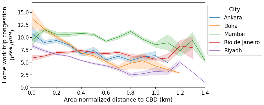
../_images/examples_USS02_CityComparison_77_0.png

[55]:

fig, ax = plotLines(
    data=df_spatial_areas,
    x='cbd_dist_bin_norm',
    y='avg_realT_frac_osmT',
    hue='City',
    hue_order=city_todo_order,
    xlabel=r'Area normalized distance to CBD (km)',
    ylabel='Home-work trip congestion\n' + r'($t^{REAL} / t^{OSM}$)',
    # title=r'Per area home-work $t^{REAL} / t^{OSRM}$ duration vs. norm. distance to CBD',
    xlim=(0,1.4),
    ylim=(0,17),
)
fig.savefig(os.path.join(OUT_FOLDER, 'home_work_duration_fraction_area_cbd_norm.pdf'), bbox_inches='tight')

../_images/examples_USS02_CityComparison_78_0.png

[56]:

fig, ax = plotLines(
    data=df_spatial_users,
    x='cbd_dist_bin',
    y='avg_realT_frac_osmT',
    hue='City',
    hue_order=city_todo_order,
    xlabel=r'User home distance to CBD (km)',
    ylabel='Home-work trip congestion\n' + r'($t^{REAL} / t^{OSM}$)',
    # title=r'Per user home-work $t^{REAL} / t^{OSRM}$ duration vs. home distance to CBD',
    xlim=(0,80),
    ylim=(0,17),
)
fig.savefig(os.path.join(OUT_FOLDER, 'home_work_duration_fraction_user_cbd.pdf'), bbox_inches='tight')

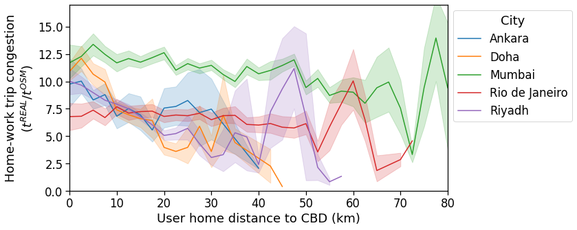
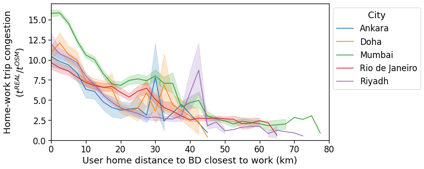
../_images/examples_USS02_CityComparison_79_0.png

Home-work duration ratio (real/osrm) vs. distance to Business District closest to workplace

[57]:

fig, ax = plotLines(
    data=df_spatial_users,
    x='closest_cbd_dist_bin',
    y='avg_realT_frac_osmT',
    hue='City',
    hue_order=city_todo_order,
    xlabel=r'User home distance to BD closest to work (km)',
    ylabel='Home-work trip congestion\n' + r'($t^{REAL} / t^{OSM}$)',
    #  title=r'Per user home-work $t^{REAL} / t^{OSRM}$ duration vs. home dist. to BD closest to workplace',
    xlim=(0,80),
    ylim=(0,17),
)
fig.savefig(os.path.join(OUT_FOLDER, 'home_work_duration_fraction_user_cbd_closest.pdf'), bbox_inches='tight')

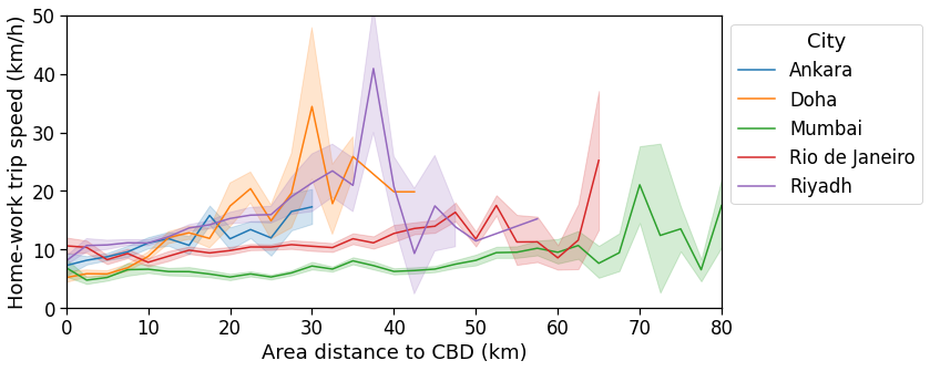
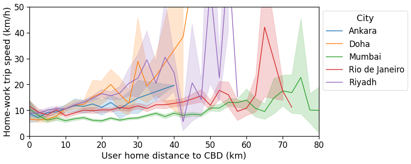
../_images/examples_USS02_CityComparison_81_0.png

Home-work travel speed vs. distance to Central Business District

[58]:

fig, ax = plotLines(
    data=df_spatial_areas,
    x='cbd_dist_bin',
    y='speed_trips_hw_avg',
    hue='City',
    hue_order=city_todo_order,
    xlabel=r'Area distance to CBD (km)',
    ylabel=r'Home-work trip speed (km/h)',
    # title=r'Per area home-work $v^{REAL}$ speed vs. norm. distance to CBD',
    xlim=(0,80),
    ylim=(0,50),
)
fig.savefig(os.path.join(OUT_FOLDER, 'home_work_speed_real_area_cbd.pdf'), bbox_inches='tight')

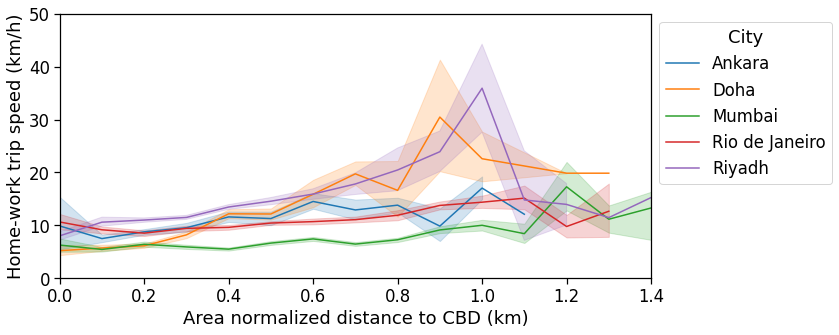
../_images/examples_USS02_CityComparison_83_0.png

[59]:

fig, ax = plotLines(
    data=df_spatial_areas,
    x='cbd_dist_bin_norm',
    y='speed_trips_hw_avg',
    hue='City',
    hue_order=city_todo_order,
    xlabel=r'Area normalized distance to CBD (km)',
    ylabel=r'Home-work trip speed (km/h)',
    # title=r'Per area home-work $v^{REAL}$ speed vs. norm. distance to CBD',
    xlim=(0,1.4),
    ylim=(0,50),
)
fig.savefig(os.path.join(OUT_FOLDER, 'home_work_speed_real_area_cbd_norm.pdf'), bbox_inches='tight')

../_images/examples_USS02_CityComparison_84_0.png

[60]:

fig, ax = plotLines(
    data=df_spatial_users,
    x='cbd_dist_bin',
    y='speed_trips_hw',
    hue='City',
    hue_order=city_todo_order,
    xlabel=r'User home distance to CBD (km)',
    ylabel=r'Home-work trip speed (km/h)',
    # title=r'Per user home-work $v^{REAL}$ speed vs. home distance to CBD',
    xlim=(0,80),
    ylim=(0,50),
)
fig.savefig(os.path.join(OUT_FOLDER, 'home_work_speed_real_user_cbd.pdf'), bbox_inches='tight')

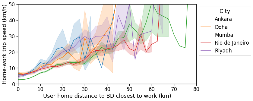
../_images/examples_USS02_CityComparison_85_0.png

Home-work travel speed vs. distance to Business District closest to workplace

[61]:

fig, ax = plotLines(
    data=df_spatial_users,
    x='closest_cbd_dist_bin',
    y='speed_trips_hw',
    hue='City',
    hue_order=city_todo_order,
    xlabel=r'User home distance to BD closest to work (km)',
    ylabel=r'Home-work trip speed (km/h)',
    # title=r'Per user home-work $v^{REAL}$ speed vs. home dist. to BD closest to workplace',
    xlim=(0,80),
    ylim=(0,50),
)
fig.savefig(os.path.join(OUT_FOLDER, 'home_work_speed_real_user_cbd_closest.pdf'), bbox_inches='tight')

../_images/examples_USS02_CityComparison_87_0.png

[ ]: