Quickstart

This is a notebook explaining the usage of the main features of mobilkit.

The features covered here are:

how to create a synthetic dataset from the Microsoft’s GeoLife dataset.
how to create a tessellation shapefile in case you only have a collection of centroid;
load data from a pandas dataframe;
tessellate the pings (assign them to a given location);
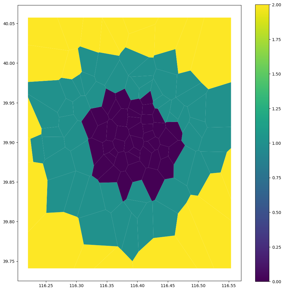
compute the land use of an urban area;
compute the resident population for each area and compare it with census figures;
compute user activity statistics and filter users accordingly;
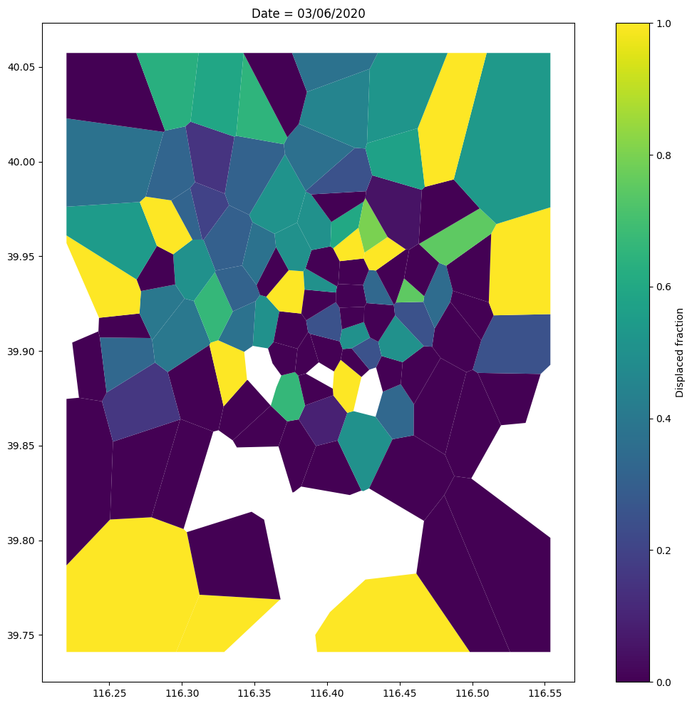
compute the displacement figures in a given area.

To allow the publication of the data we used an open dataset such as the GeoLife one. We augment the number of users observed by using some functions present in the mobilkit.loader module.

Depending on the case we map each user/day or each user/week to a synthetic user performing the same events as in the original dataset at the same original time, just traslating everything in the synthetic day or week..

To continue you have to download the GeoLife dataset and uncompress it in the data directory.

[1]:

%config Completer.use_jedi = False
%matplotlib inline

import pytz
from datetime import datetime
import geopandas as gpd

import numpy as np
import matplotlib.pyplot as plt
import pandas as pd
import seaborn as sns

import mobilkit
from dask.distributed import Client
from shapely.geometry import Polygon, Point
from dask import dataframe as dd

import warnings
warnings.filterwarnings('ignore')

import mobilkit

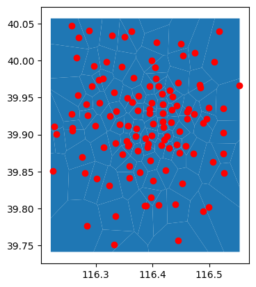
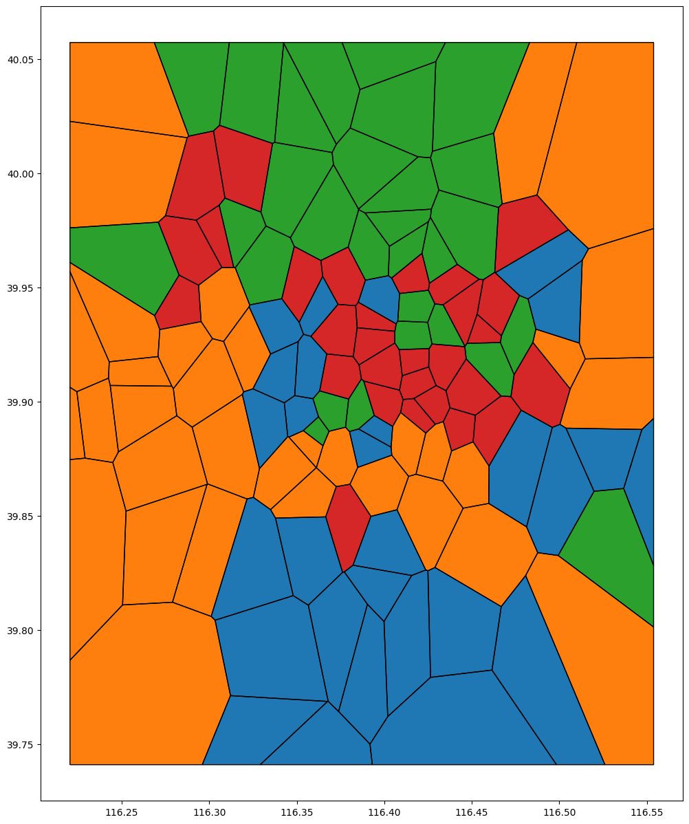
Create tessellation from points

I use the file with centroids found here, select some points in Beijing and create a Voronoi tessellation of it.

[2]:

# Choose the spatial extent of your analysis and where to save the Vortonoi tessellation
box = (116.20, 39.74, 116.56, 40.06)
voronoi_file = "../../data/Beijing/voronoi_points_beijing.shp"

df_china = gpd.read_file("../../data/Beijing/DT19new/PopCensus2010_township.shp")
if not os.path.exists(voronoi_file):
    poly_box = mobilkit.spatial.box2poly(box)
    df_china = df_china[df_china.within(poly_box)]
    poly_gdf = gpd.GeoDataFrame(["Region"], geometry=[poly_box], crs=df_china.crs)
    layer = mobilkit.spatial.makeVoronoi(df_china)
    layer.to_file(voronoi_file)
else:
    layer = gpd.read_file(voronoi_file)
    box = layer.unary_union.bounds
    poly_box = mobilkit.spatial.box2poly(box)
    df_china = df_china[df_china.within(poly_box)]

[3]:

ax = layer.plot()
df_china.plot(color="r", ax=ax)

[3]:

<Axes: >

../_images/examples_mobilkit_tutorial_4_1.png

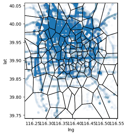
Load/reload the geolife trajectories data

You should manually download the data from here and put them into to data/ folder and unzip them there.

cd ../data/
wget https://download.microsoft.com/download/F/4/8/F4894AA5-FDBC-481E-9285-D5F8C4C4F039/Geolife%20Trajectories%201.3.zip
unzip Geolife%20Trajectories%201.3.zip

[4]:

# !wget -P ../../data/ https://download.microsoft.com/download/F/4/8/F4894AA5-FDBC-481E-9285-D5F8C4C4F039/Geolife%20Trajectories%201.3.zip
# !unzip -d ../../data/ ../../data/Geolife\ Trajectories\ 1.3.zip

[5]:

geolifePath = "../../data/Geolife Trajectories 1.3"
pkl_trajectories = "../../data/Geolife Trajectories 1.3/processed_traj.pkl"
if not os.path.exists(pkl_trajectories):
    df_geolife = mobilkit.loader.loadGeolifeData(geolifePath)
    df_geolife.to_pickle(pkl_trajectories)
else:
    df_geolife = pd.read_pickle(pkl_trajectories)

df_geolife.head()

[5]:

	UTC	acc	datetime	lat	lng
0	1224730384	1	2008-10-23 10:53:04+08:00	39.984702	116.318417
1	1224730390	1	2008-10-23 10:53:10+08:00	39.984683	116.318450
2	1224730395	1	2008-10-23 10:53:15+08:00	39.984686	116.318417
3	1224730400	1	2008-10-23 10:53:20+08:00	39.984688	116.318385
4	1224730405	1	2008-10-23 10:53:25+08:00	39.984655	116.318263

Create synthetic days/week from the data

We perform two expansion of the data: - a weekly one, where each (user,week) couple is treated as a separate user and all the events are moved to a synthetic week keeping the original weekday, hour, minute and second of the recorded point; - a daily one, where each (user,day) couple is treated as a separate user and all the events are moved to a synthetic day keeping the original hour, minute and second of the recorded point;

[6]:

# One day with all the data projected to a single day
selected_day = datetime(2020, 6, 1, tzinfo=pytz.timezone("UTC"))
df_users_day = mobilkit.loader.syntheticGeoLifeDay(df_geolife, selected_day=selected_day)
df_users_day["uid"].nunique()

[6]:

[7]:

# One week with all the data projected to a single week
selected_week = datetime(2020, 6, 4, tzinfo=pytz.timezone("UTC"))
df_users_week = mobilkit.loader.syntheticGeoLifeWeek(df_geolife, selected_week=selected_week)
df_users_week["uid"].nunique()

Anticipated the date to Monday:  2020-06-01 00:00:00+00:00

[7]:

We now have two dataframes containing our data.

Each row is an event containing the spatial and temporal information.

[8]:

df_users_week.head(4)

[8]:

	UTC	acc	datetime	lat	lng
0	1591267984	1	2020-06-04 10:53:04+00:00	39.984702	116.318417
1	1591267990	1	2020-06-04 10:53:10+00:00	39.984683	116.318450
2	1591267995	1	2020-06-04 10:53:15+00:00	39.984686	116.318417
3	1591268000	1	2020-06-04 10:53:20+00:00	39.984688	116.318385

[9]:

# Get a small fraction of the pings and see how they are distributed over the tessellation
ax = df_users_day.sample(frac=.01).plot("lng","lat",kind="scatter", alpha=.01)
ax = layer.plot(color="none", edgecolor="k", ax=ax)

box = layer.unary_union.bounds
plt.xlim(box[0], box[2])
plt.ylim(box[1], box[3])

[9]:

(39.74096801500008, 40.05733690900007)

../_images/examples_mobilkit_tutorial_13_1.png

Create dask client

Launch worker and scheduler if working on localhost with:

dask-worker 127.0.0.1:8786 --nworkers -1 & dask-scheduler

If you get an error with Popen in dask-worker, add the option --preload-nanny multiprocessing.popen_spawn_posix to the first command.

[10]:

client = Client(address="127.0.0.1:8786")
client

[10]:

Client

Client-ed631bd2-0f93-11ee-97cc-63c186d89b62

Connection method: Direct
Dashboard: http://127.0.0.1:8787/status

Scheduler Info

Scheduler

Scheduler-19415a23-7a4e-4501-a545-b2a63b4d907a

Comm: tcp://192.168.1.20:8786	Workers: 48
Dashboard: http://192.168.1.20:8787/status	Total threads: 48
Started: 18 minutes ago	Total memory: 188.55 GiB

Workers

Worker: tcp://127.0.0.1:33061

Comm: tcp://127.0.0.1:33061	Total threads: 1
Dashboard: http://127.0.0.1:42417/status	Memory: 3.93 GiB
Nanny: tcp://127.0.0.1:33353
Local directory: /tmp/dask-scratch-space/worker-r12h7jeq
Tasks executing:	Tasks in memory:
Tasks ready:	Tasks in flight:
CPU usage: 2.0%	Last seen: Just now
Memory usage: 434.76 MiB	Spilled bytes: 0 B
Read bytes: 88.92 kiB	Write bytes: 89.51 kiB

Worker: tcp://127.0.0.1:33673

Comm: tcp://127.0.0.1:33673	Total threads: 1
Dashboard: http://127.0.0.1:44469/status	Memory: 3.93 GiB
Nanny: tcp://127.0.0.1:35049
Local directory: /tmp/dask-scratch-space/worker-s5arlujv
Tasks executing:	Tasks in memory:
Tasks ready:	Tasks in flight:
CPU usage: 2.0%	Last seen: Just now
Memory usage: 412.54 MiB	Spilled bytes: 0 B
Read bytes: 21.80 kiB	Write bytes: 22.28 kiB

Worker: tcp://127.0.0.1:34243

Comm: tcp://127.0.0.1:34243	Total threads: 1
Dashboard: http://127.0.0.1:45703/status	Memory: 3.93 GiB
Nanny: tcp://127.0.0.1:41873
Local directory: /tmp/dask-scratch-space/worker-bneglcv5
Tasks executing:	Tasks in memory:
Tasks ready:	Tasks in flight:
CPU usage: 2.0%	Last seen: Just now
Memory usage: 469.80 MiB	Spilled bytes: 0 B
Read bytes: 60.33 kiB	Write bytes: 61.13 kiB

Worker: tcp://127.0.0.1:34473

Comm: tcp://127.0.0.1:34473	Total threads: 1
Dashboard: http://127.0.0.1:40907/status	Memory: 3.93 GiB
Nanny: tcp://127.0.0.1:36857
Local directory: /tmp/dask-scratch-space/worker-4u4p74rg
Tasks executing:	Tasks in memory:
Tasks ready:	Tasks in flight:
CPU usage: 2.0%	Last seen: Just now
Memory usage: 341.86 MiB	Spilled bytes: 0 B
Read bytes: 45.54 kiB	Write bytes: 45.40 kiB

Worker: tcp://127.0.0.1:34759

Comm: tcp://127.0.0.1:34759	Total threads: 1
Dashboard: http://127.0.0.1:37909/status	Memory: 3.93 GiB
Nanny: tcp://127.0.0.1:37765
Local directory: /tmp/dask-scratch-space/worker-lqyevwi_
Tasks executing:	Tasks in memory:
Tasks ready:	Tasks in flight:
CPU usage: 2.0%	Last seen: Just now
Memory usage: 503.96 MiB	Spilled bytes: 0 B
Read bytes: 90.25 kiB	Write bytes: 90.85 kiB

Worker: tcp://127.0.0.1:35245

Comm: tcp://127.0.0.1:35245	Total threads: 1
Dashboard: http://127.0.0.1:39519/status	Memory: 3.93 GiB
Nanny: tcp://127.0.0.1:44891
Local directory: /tmp/dask-scratch-space/worker-z1a38btj
Tasks executing:	Tasks in memory:
Tasks ready:	Tasks in flight:
CPU usage: 2.0%	Last seen: Just now
Memory usage: 404.91 MiB	Spilled bytes: 0 B
Read bytes: 57.19 kiB	Write bytes: 57.98 kiB

Worker: tcp://127.0.0.1:36047

Comm: tcp://127.0.0.1:36047	Total threads: 1
Dashboard: http://127.0.0.1:36449/status	Memory: 3.93 GiB
Nanny: tcp://127.0.0.1:34021
Local directory: /tmp/dask-scratch-space/worker-88p660z1
Tasks executing:	Tasks in memory:
Tasks ready:	Tasks in flight:
CPU usage: 2.0%	Last seen: Just now
Memory usage: 439.95 MiB	Spilled bytes: 0 B
Read bytes: 38.67 kiB	Write bytes: 38.53 kiB

Worker: tcp://127.0.0.1:36421

Comm: tcp://127.0.0.1:36421	Total threads: 1
Dashboard: http://127.0.0.1:39449/status	Memory: 3.93 GiB
Nanny: tcp://127.0.0.1:41417
Local directory: /tmp/dask-scratch-space/worker-_990tl15
Tasks executing:	Tasks in memory:
Tasks ready:	Tasks in flight:
CPU usage: 0.0%	Last seen: Just now
Memory usage: 519.66 MiB	Spilled bytes: 0 B
Read bytes: 96.51 kiB	Write bytes: 97.10 kiB

Worker: tcp://127.0.0.1:36667

Comm: tcp://127.0.0.1:36667	Total threads: 1
Dashboard: http://127.0.0.1:34335/status	Memory: 3.93 GiB
Nanny: tcp://127.0.0.1:42983
Local directory: /tmp/dask-scratch-space/worker-ydyoh6ee
Tasks executing:	Tasks in memory:
Tasks ready:	Tasks in flight:
CPU usage: 2.0%	Last seen: Just now
Memory usage: 399.44 MiB	Spilled bytes: 0 B
Read bytes: 27.72 kiB	Write bytes: 27.58 kiB

Worker: tcp://127.0.0.1:36765

Comm: tcp://127.0.0.1:36765	Total threads: 1
Dashboard: http://127.0.0.1:42401/status	Memory: 3.93 GiB
Nanny: tcp://127.0.0.1:35995
Local directory: /tmp/dask-scratch-space/worker-a084fgc3
Tasks executing:	Tasks in memory:
Tasks ready:	Tasks in flight:
CPU usage: 2.0%	Last seen: Just now
Memory usage: 483.52 MiB	Spilled bytes: 0 B
Read bytes: 87.16 kiB	Write bytes: 87.76 kiB

Worker: tcp://127.0.0.1:36769

Comm: tcp://127.0.0.1:36769	Total threads: 1
Dashboard: http://127.0.0.1:34913/status	Memory: 3.93 GiB
Nanny: tcp://127.0.0.1:44139
Local directory: /tmp/dask-scratch-space/worker-72fa7jpu
Tasks executing:	Tasks in memory:
Tasks ready:	Tasks in flight:
CPU usage: 2.0%	Last seen: Just now
Memory usage: 360.64 MiB	Spilled bytes: 0 B
Read bytes: 47.68 kiB	Write bytes: 47.39 kiB

Worker: tcp://127.0.0.1:37607

Comm: tcp://127.0.0.1:37607	Total threads: 1
Dashboard: http://127.0.0.1:36365/status	Memory: 3.93 GiB
Nanny: tcp://127.0.0.1:39637
Local directory: /tmp/dask-scratch-space/worker-s8829bvw
Tasks executing:	Tasks in memory:
Tasks ready:	Tasks in flight:
CPU usage: 0.0%	Last seen: Just now
Memory usage: 379.50 MiB	Spilled bytes: 0 B
Read bytes: 37.43 kiB	Write bytes: 37.29 kiB

Worker: tcp://127.0.0.1:38207

Comm: tcp://127.0.0.1:38207	Total threads: 1
Dashboard: http://127.0.0.1:36223/status	Memory: 3.93 GiB
Nanny: tcp://127.0.0.1:45579
Local directory: /tmp/dask-scratch-space/worker-rfmownb0
Tasks executing:	Tasks in memory:
Tasks ready:	Tasks in flight:
CPU usage: 2.0%	Last seen: Just now
Memory usage: 509.14 MiB	Spilled bytes: 0 B
Read bytes: 25.77 kiB	Write bytes: 25.63 kiB

Worker: tcp://127.0.0.1:38387

Comm: tcp://127.0.0.1:38387	Total threads: 1
Dashboard: http://127.0.0.1:34409/status	Memory: 3.93 GiB
Nanny: tcp://127.0.0.1:35175
Local directory: /tmp/dask-scratch-space/worker-y1l_4piy
Tasks executing:	Tasks in memory:
Tasks ready:	Tasks in flight:
CPU usage: 2.0%	Last seen: Just now
Memory usage: 400.66 MiB	Spilled bytes: 0 B
Read bytes: 58.84 kiB	Write bytes: 59.64 kiB

Worker: tcp://127.0.0.1:38389

Comm: tcp://127.0.0.1:38389	Total threads: 1
Dashboard: http://127.0.0.1:42719/status	Memory: 3.93 GiB
Nanny: tcp://127.0.0.1:42211
Local directory: /tmp/dask-scratch-space/worker-fxsg7_yh
Tasks executing:	Tasks in memory:
Tasks ready:	Tasks in flight:
CPU usage: 2.0%	Last seen: Just now
Memory usage: 421.97 MiB	Spilled bytes: 0 B
Read bytes: 22.62 kiB	Write bytes: 22.48 kiB

Worker: tcp://127.0.0.1:38749

Comm: tcp://127.0.0.1:38749	Total threads: 1
Dashboard: http://127.0.0.1:39495/status	Memory: 3.93 GiB
Nanny: tcp://127.0.0.1:32801
Local directory: /tmp/dask-scratch-space/worker-p5jrdspb
Tasks executing:	Tasks in memory:
Tasks ready:	Tasks in flight:
CPU usage: 2.0%	Last seen: Just now
Memory usage: 361.07 MiB	Spilled bytes: 0 B
Read bytes: 79.55 kiB	Write bytes: 80.15 kiB

Worker: tcp://127.0.0.1:39063

Comm: tcp://127.0.0.1:39063	Total threads: 1
Dashboard: http://127.0.0.1:44649/status	Memory: 3.93 GiB
Nanny: tcp://127.0.0.1:32959
Local directory: /tmp/dask-scratch-space/worker-9gxew3ha
Tasks executing:	Tasks in memory:
Tasks ready:	Tasks in flight:
CPU usage: 2.0%	Last seen: Just now
Memory usage: 450.54 MiB	Spilled bytes: 0 B
Read bytes: 29.03 kiB	Write bytes: 28.89 kiB

Worker: tcp://127.0.0.1:39107

Comm: tcp://127.0.0.1:39107	Total threads: 1
Dashboard: http://127.0.0.1:45405/status	Memory: 3.93 GiB
Nanny: tcp://127.0.0.1:41081
Local directory: /tmp/dask-scratch-space/worker-asqqrdqf
Tasks executing:	Tasks in memory:
Tasks ready:	Tasks in flight:
CPU usage: 2.0%	Last seen: Just now
Memory usage: 396.77 MiB	Spilled bytes: 0 B
Read bytes: 84.36 kiB	Write bytes: 84.96 kiB

Worker: tcp://127.0.0.1:39215

Comm: tcp://127.0.0.1:39215	Total threads: 1
Dashboard: http://127.0.0.1:40273/status	Memory: 3.93 GiB
Nanny: tcp://127.0.0.1:42749
Local directory: /tmp/dask-scratch-space/worker-9kdkwdsr
Tasks executing:	Tasks in memory:
Tasks ready:	Tasks in flight:
CPU usage: 2.0%	Last seen: Just now
Memory usage: 414.57 MiB	Spilled bytes: 0 B
Read bytes: 84.69 kiB	Write bytes: 85.29 kiB

Worker: tcp://127.0.0.1:40037

Comm: tcp://127.0.0.1:40037	Total threads: 1
Dashboard: http://127.0.0.1:35931/status	Memory: 3.93 GiB
Nanny: tcp://127.0.0.1:42683
Local directory: /tmp/dask-scratch-space/worker-ssx075ud
Tasks executing:	Tasks in memory:
Tasks ready:	Tasks in flight:
CPU usage: 2.0%	Last seen: Just now
Memory usage: 424.18 MiB	Spilled bytes: 0 B
Read bytes: 93.57 kiB	Write bytes: 94.17 kiB

Worker: tcp://127.0.0.1:40175

Comm: tcp://127.0.0.1:40175	Total threads: 1
Dashboard: http://127.0.0.1:39195/status	Memory: 3.93 GiB
Nanny: tcp://127.0.0.1:46365
Local directory: /tmp/dask-scratch-space/worker-636uq6z1
Tasks executing:	Tasks in memory:
Tasks ready:	Tasks in flight:
CPU usage: 2.0%	Last seen: Just now
Memory usage: 362.13 MiB	Spilled bytes: 0 B
Read bytes: 61.08 kiB	Write bytes: 61.68 kiB

Worker: tcp://127.0.0.1:40259

Comm: tcp://127.0.0.1:40259	Total threads: 1
Dashboard: http://127.0.0.1:36019/status	Memory: 3.93 GiB
Nanny: tcp://127.0.0.1:33883
Local directory: /tmp/dask-scratch-space/worker-tqzry7i6
Tasks executing:	Tasks in memory:
Tasks ready:	Tasks in flight:
CPU usage: 2.0%	Last seen: Just now
Memory usage: 503.07 MiB	Spilled bytes: 0 B
Read bytes: 43.87 kiB	Write bytes: 43.73 kiB

Worker: tcp://127.0.0.1:40895

Comm: tcp://127.0.0.1:40895	Total threads: 1
Dashboard: http://127.0.0.1:42945/status	Memory: 3.93 GiB
Nanny: tcp://127.0.0.1:44851
Local directory: /tmp/dask-scratch-space/worker-nzdzwzqk
Tasks executing:	Tasks in memory:
Tasks ready:	Tasks in flight:
CPU usage: 2.0%	Last seen: Just now
Memory usage: 455.16 MiB	Spilled bytes: 0 B
Read bytes: 40.35 kiB	Write bytes: 40.21 kiB

Worker: tcp://127.0.0.1:40943

Comm: tcp://127.0.0.1:40943	Total threads: 1
Dashboard: http://127.0.0.1:36525/status	Memory: 3.93 GiB
Nanny: tcp://127.0.0.1:39021
Local directory: /tmp/dask-scratch-space/worker-k66o5m6d
Tasks executing:	Tasks in memory:
Tasks ready:	Tasks in flight:
CPU usage: 2.0%	Last seen: Just now
Memory usage: 375.66 MiB	Spilled bytes: 0 B
Read bytes: 88.78 kiB	Write bytes: 89.38 kiB

Worker: tcp://127.0.0.1:40971

Comm: tcp://127.0.0.1:40971	Total threads: 1
Dashboard: http://127.0.0.1:40935/status	Memory: 3.93 GiB
Nanny: tcp://127.0.0.1:44031
Local directory: /tmp/dask-scratch-space/worker-6vxt3tl1
Tasks executing:	Tasks in memory:
Tasks ready:	Tasks in flight:
CPU usage: 0.0%	Last seen: Just now
Memory usage: 487.20 MiB	Spilled bytes: 0 B
Read bytes: 65.92 kiB	Write bytes: 66.52 kiB

Worker: tcp://127.0.0.1:41117

Comm: tcp://127.0.0.1:41117	Total threads: 1
Dashboard: http://127.0.0.1:46605/status	Memory: 3.93 GiB
Nanny: tcp://127.0.0.1:37421
Local directory: /tmp/dask-scratch-space/worker-92anioeb
Tasks executing:	Tasks in memory:
Tasks ready:	Tasks in flight:
CPU usage: 4.0%	Last seen: Just now
Memory usage: 415.42 MiB	Spilled bytes: 0 B
Read bytes: 35.45 kiB	Write bytes: 35.31 kiB

Worker: tcp://127.0.0.1:41267

Comm: tcp://127.0.0.1:41267	Total threads: 1
Dashboard: http://127.0.0.1:36419/status	Memory: 3.93 GiB
Nanny: tcp://127.0.0.1:33383
Local directory: /tmp/dask-scratch-space/worker-9wp3do47
Tasks executing:	Tasks in memory:
Tasks ready:	Tasks in flight:
CPU usage: 4.0%	Last seen: Just now
Memory usage: 436.40 MiB	Spilled bytes: 0 B
Read bytes: 85.92 kiB	Write bytes: 86.52 kiB

Worker: tcp://127.0.0.1:41391

Comm: tcp://127.0.0.1:41391	Total threads: 1
Dashboard: http://127.0.0.1:33513/status	Memory: 3.93 GiB
Nanny: tcp://127.0.0.1:46637
Local directory: /tmp/dask-scratch-space/worker-o9gu0xbx
Tasks executing:	Tasks in memory:
Tasks ready:	Tasks in flight:
CPU usage: 4.0%	Last seen: Just now
Memory usage: 363.50 MiB	Spilled bytes: 0 B
Read bytes: 53.33 kiB	Write bytes: 51.74 kiB

Worker: tcp://127.0.0.1:41457

Comm: tcp://127.0.0.1:41457	Total threads: 1
Dashboard: http://127.0.0.1:42281/status	Memory: 3.93 GiB
Nanny: tcp://127.0.0.1:45053
Local directory: /tmp/dask-scratch-space/worker-bsdv0ff5
Tasks executing:	Tasks in memory:
Tasks ready:	Tasks in flight:
CPU usage: 0.0%	Last seen: Just now
Memory usage: 494.88 MiB	Spilled bytes: 0 B
Read bytes: 62.37 kiB	Write bytes: 62.97 kiB

Worker: tcp://127.0.0.1:42041

Comm: tcp://127.0.0.1:42041	Total threads: 1
Dashboard: http://127.0.0.1:41729/status	Memory: 3.93 GiB
Nanny: tcp://127.0.0.1:44953
Local directory: /tmp/dask-scratch-space/worker-hv98qnhl
Tasks executing:	Tasks in memory:
Tasks ready:	Tasks in flight:
CPU usage: 2.0%	Last seen: Just now
Memory usage: 330.66 MiB	Spilled bytes: 0 B
Read bytes: 32.66 kiB	Write bytes: 32.52 kiB

Worker: tcp://127.0.0.1:42311

Comm: tcp://127.0.0.1:42311	Total threads: 1
Dashboard: http://127.0.0.1:42045/status	Memory: 3.93 GiB
Nanny: tcp://127.0.0.1:44311
Local directory: /tmp/dask-scratch-space/worker-9vml91gr
Tasks executing:	Tasks in memory:
Tasks ready:	Tasks in flight:
CPU usage: 2.0%	Last seen: Just now
Memory usage: 414.96 MiB	Spilled bytes: 0 B
Read bytes: 88.75 kiB	Write bytes: 89.35 kiB

Worker: tcp://127.0.0.1:42643

Comm: tcp://127.0.0.1:42643	Total threads: 1
Dashboard: http://127.0.0.1:40399/status	Memory: 3.93 GiB
Nanny: tcp://127.0.0.1:44141
Local directory: /tmp/dask-scratch-space/worker-7v7xi_zz
Tasks executing:	Tasks in memory:
Tasks ready:	Tasks in flight:
CPU usage: 0.0%	Last seen: Just now
Memory usage: 499.41 MiB	Spilled bytes: 0 B
Read bytes: 69.18 kiB	Write bytes: 69.78 kiB

Worker: tcp://127.0.0.1:42707

Comm: tcp://127.0.0.1:42707	Total threads: 1
Dashboard: http://127.0.0.1:35825/status	Memory: 3.93 GiB
Nanny: tcp://127.0.0.1:32839
Local directory: /tmp/dask-scratch-space/worker-8hxynz67
Tasks executing:	Tasks in memory:
Tasks ready:	Tasks in flight:
CPU usage: 2.0%	Last seen: Just now
Memory usage: 442.02 MiB	Spilled bytes: 0 B
Read bytes: 51.71 kiB	Write bytes: 50.13 kiB

Worker: tcp://127.0.0.1:42937

Comm: tcp://127.0.0.1:42937	Total threads: 1
Dashboard: http://127.0.0.1:41125/status	Memory: 3.93 GiB
Nanny: tcp://127.0.0.1:42879
Local directory: /tmp/dask-scratch-space/worker-pck0v5cq
Tasks executing:	Tasks in memory:
Tasks ready:	Tasks in flight:
CPU usage: 0.0%	Last seen: Just now
Memory usage: 486.73 MiB	Spilled bytes: 0 B
Read bytes: 93.77 kiB	Write bytes: 94.37 kiB

Worker: tcp://127.0.0.1:43321

Comm: tcp://127.0.0.1:43321	Total threads: 1
Dashboard: http://127.0.0.1:37537/status	Memory: 3.93 GiB
Nanny: tcp://127.0.0.1:38345
Local directory: /tmp/dask-scratch-space/worker-1z4_uqta
Tasks executing:	Tasks in memory:
Tasks ready:	Tasks in flight:
CPU usage: 2.0%	Last seen: Just now
Memory usage: 422.61 MiB	Spilled bytes: 0 B
Read bytes: 42.24 kiB	Write bytes: 42.10 kiB

Worker: tcp://127.0.0.1:43335

Comm: tcp://127.0.0.1:43335	Total threads: 1
Dashboard: http://127.0.0.1:40561/status	Memory: 3.93 GiB
Nanny: tcp://127.0.0.1:46705
Local directory: /tmp/dask-scratch-space/worker-j8wpunjg
Tasks executing:	Tasks in memory:
Tasks ready:	Tasks in flight:
CPU usage: 2.0%	Last seen: Just now
Memory usage: 421.68 MiB	Spilled bytes: 0 B
Read bytes: 24.19 kiB	Write bytes: 24.05 kiB

Worker: tcp://127.0.0.1:43655

Comm: tcp://127.0.0.1:43655	Total threads: 1
Dashboard: http://127.0.0.1:41059/status	Memory: 3.93 GiB
Nanny: tcp://127.0.0.1:37321
Local directory: /tmp/dask-scratch-space/worker-57q_3n0w
Tasks executing:	Tasks in memory:
Tasks ready:	Tasks in flight:
CPU usage: 0.0%	Last seen: Just now
Memory usage: 507.19 MiB	Spilled bytes: 0 B
Read bytes: 83.08 kiB	Write bytes: 83.68 kiB

Worker: tcp://127.0.0.1:43735

Comm: tcp://127.0.0.1:43735	Total threads: 1
Dashboard: http://127.0.0.1:34755/status	Memory: 3.93 GiB
Nanny: tcp://127.0.0.1:36489
Local directory: /tmp/dask-scratch-space/worker-dk5fqm1b
Tasks executing:	Tasks in memory:
Tasks ready:	Tasks in flight:
CPU usage: 2.0%	Last seen: Just now
Memory usage: 450.47 MiB	Spilled bytes: 0 B
Read bytes: 69.25 kiB	Write bytes: 69.85 kiB

Worker: tcp://127.0.0.1:43811

Comm: tcp://127.0.0.1:43811	Total threads: 1
Dashboard: http://127.0.0.1:46041/status	Memory: 3.93 GiB
Nanny: tcp://127.0.0.1:36853
Local directory: /tmp/dask-scratch-space/worker-ldw_92u5
Tasks executing:	Tasks in memory:
Tasks ready:	Tasks in flight:
CPU usage: 2.0%	Last seen: Just now
Memory usage: 410.17 MiB	Spilled bytes: 0 B
Read bytes: 91.74 kiB	Write bytes: 92.34 kiB

Worker: tcp://127.0.0.1:44171

Comm: tcp://127.0.0.1:44171	Total threads: 1
Dashboard: http://127.0.0.1:45009/status	Memory: 3.93 GiB
Nanny: tcp://127.0.0.1:37799
Local directory: /tmp/dask-scratch-space/worker-_72pnvii
Tasks executing:	Tasks in memory:
Tasks ready:	Tasks in flight:
CPU usage: 2.0%	Last seen: Just now
Memory usage: 457.95 MiB	Spilled bytes: 0 B
Read bytes: 30.67 kiB	Write bytes: 30.52 kiB

Worker: tcp://127.0.0.1:44691

Comm: tcp://127.0.0.1:44691	Total threads: 1
Dashboard: http://127.0.0.1:44787/status	Memory: 3.93 GiB
Nanny: tcp://127.0.0.1:34333
Local directory: /tmp/dask-scratch-space/worker-wvd04iar
Tasks executing:	Tasks in memory:
Tasks ready:	Tasks in flight:
CPU usage: 2.0%	Last seen: Just now
Memory usage: 498.45 MiB	Spilled bytes: 0 B
Read bytes: 72.28 kiB	Write bytes: 72.88 kiB

Worker: tcp://127.0.0.1:44913

Comm: tcp://127.0.0.1:44913	Total threads: 1
Dashboard: http://127.0.0.1:45675/status	Memory: 3.93 GiB
Nanny: tcp://127.0.0.1:42331
Local directory: /tmp/dask-scratch-space/worker-w7i24zia
Tasks executing:	Tasks in memory:
Tasks ready:	Tasks in flight:
CPU usage: 2.0%	Last seen: Just now
Memory usage: 428.10 MiB	Spilled bytes: 0 B
Read bytes: 72.78 kiB	Write bytes: 73.37 kiB

Worker: tcp://127.0.0.1:45061

Comm: tcp://127.0.0.1:45061	Total threads: 1
Dashboard: http://127.0.0.1:35047/status	Memory: 3.93 GiB
Nanny: tcp://127.0.0.1:39355
Local directory: /tmp/dask-scratch-space/worker-6gc4lwdh
Tasks executing:	Tasks in memory:
Tasks ready:	Tasks in flight:
CPU usage: 2.0%	Last seen: Just now
Memory usage: 445.23 MiB	Spilled bytes: 0 B
Read bytes: 79.51 kiB	Write bytes: 80.11 kiB

Worker: tcp://127.0.0.1:45349

Comm: tcp://127.0.0.1:45349	Total threads: 1
Dashboard: http://127.0.0.1:34555/status	Memory: 3.93 GiB
Nanny: tcp://127.0.0.1:41015
Local directory: /tmp/dask-scratch-space/worker-s8l5kjwe
Tasks executing:	Tasks in memory:
Tasks ready:	Tasks in flight:
CPU usage: 4.0%	Last seen: Just now
Memory usage: 476.23 MiB	Spilled bytes: 0 B
Read bytes: 76.60 kiB	Write bytes: 77.20 kiB

Worker: tcp://127.0.0.1:45523

Comm: tcp://127.0.0.1:45523	Total threads: 1
Dashboard: http://127.0.0.1:36605/status	Memory: 3.93 GiB
Nanny: tcp://127.0.0.1:46797
Local directory: /tmp/dask-scratch-space/worker-9c43joay
Tasks executing:	Tasks in memory:
Tasks ready:	Tasks in flight:
CPU usage: 2.0%	Last seen: Just now
Memory usage: 459.50 MiB	Spilled bytes: 0 B
Read bytes: 76.52 kiB	Write bytes: 77.12 kiB

Worker: tcp://127.0.0.1:46139

Comm: tcp://127.0.0.1:46139	Total threads: 1
Dashboard: http://127.0.0.1:43055/status	Memory: 3.93 GiB
Nanny: tcp://127.0.0.1:41489
Local directory: /tmp/dask-scratch-space/worker-j_bablof
Tasks executing:	Tasks in memory:
Tasks ready:	Tasks in flight:
CPU usage: 0.0%	Last seen: Just now
Memory usage: 390.72 MiB	Spilled bytes: 0 B
Read bytes: 66.25 kiB	Write bytes: 66.85 kiB

Worker: tcp://127.0.0.1:46807

Comm: tcp://127.0.0.1:46807	Total threads: 1
Dashboard: http://127.0.0.1:46333/status	Memory: 3.93 GiB
Nanny: tcp://127.0.0.1:38421
Local directory: /tmp/dask-scratch-space/worker-g0hp9pon
Tasks executing:	Tasks in memory:
Tasks ready:	Tasks in flight:
CPU usage: 2.0%	Last seen: Just now
Memory usage: 451.67 MiB	Spilled bytes: 0 B
Read bytes: 34.25 kiB	Write bytes: 34.11 kiB

Worker: tcp://127.0.0.1:46859

Comm: tcp://127.0.0.1:46859	Total threads: 1
Dashboard: http://127.0.0.1:44231/status	Memory: 3.93 GiB
Nanny: tcp://127.0.0.1:36011
Local directory: /tmp/dask-scratch-space/worker-lz4ifeiu
Tasks executing:	Tasks in memory:
Tasks ready:	Tasks in flight:
CPU usage: 2.0%	Last seen: Just now
Memory usage: 169.81 MiB	Spilled bytes: 0 B
Read bytes: 64.28 kiB	Write bytes: 64.87 kiB

Load events in dask

Here we use the dask API, see the loader module on how to load pings from raw files.

[11]:

dd_users_raw = dd.from_pandas(df_users_day, npartitions=20)
dd_week_raw = dd.from_pandas(df_users_week, npartitions=20)

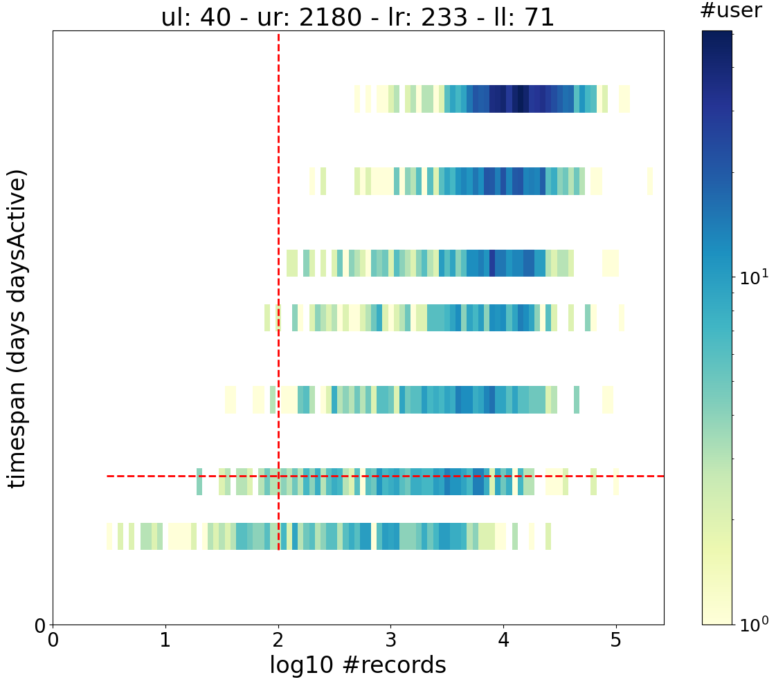
Compute user stats

We first focus on the weekly dataframe because it has more than one day (but less users).

We show here how to compute the basic user stats.

You can see the mobilkit.stats.userStats documentation for details but we get back some basic stats for each user.

[12]:

# Use the .compute() to make it a pandas df
users_stats_df = mobilkit.stats.userStats(dd_week_raw).compute()
users_stats_df.head(4)

[12]:

	uid	min_day	max_day	pings	daysActive	daysSpanned	pingsPerDay	avg
0	82	2020-06-01 00:00:00+00:00	2020-06-07 00:00:00+00:00	14027	7	6	[779, 1814, 790, 1848, 852, 2096, 5848]	2003.857143
1	102	2020-06-01 00:00:00+00:00	2020-06-07 00:00:00+00:00	16598	7	6	[641, 2493, 3853, 1181, 2695, 2251, 3484]	2371.142857
2	111	2020-06-01 00:00:00+00:00	2020-06-07 00:00:00+00:00	11562	7	6	[1165, 1124, 1038, 1001, 2203, 1453, 3578]	1651.714286
3	141	2020-06-03 00:00:00+00:00	2020-06-06 00:00:00+00:00	3909	3	3	[218, 932, 2759]	1303.000000

[13]:

# We can plot the distribution of the number of pings and active days to see how many users we have in each quadrant
mobilkit.stats.plotUsersHist(users_stats_df, min_pings=100, min_days=2)

[13]:

<Axes: title={'center': 'ul: 40 - ur: 2180 - lr: 233 - ll: 71'}, xlabel='log10 #records', ylabel='timespan (days daysActive)'>

../_images/examples_mobilkit_tutorial_20_1.png

Filter users based on stats

We want to keep only users with at least 2 active days and 100 pings.

[14]:

# We either provide users filtering by hand
valid_users = list(users_stats_df.query("daysActive >= 2 & pings > 100")["uid"])
df_filtered = mobilkit.stats.filterUsersFromSet(dd_week_raw, users_set=valid_users)

[15]:

# Or we could have had the stats and filter computed at once
df_filtered, users_stats_df, valid_users = mobilkit.stats.filterUsers(dd_week_raw, minPings=100, minDaysActive=2)

Assign pings to an area

We first assign each ping to a given area passing the name of the shapefile to use.

With filterAreas=True we are discarding all the events that fall outside of our ROI.

[16]:

dd_week_with_zones, tessellation_gdf = mobilkit.spatial.tessellate(df_filtered,
                                                                   tesselation_shp=voronoi_file,
                                                                   filterAreas=True)

Compute home and work areas

Once we have each ping assigned to a given area, we can sort out the home and work areas of each user by looking where he spends most of the time during day and night-time.

We first add the isHome and isWork columns, then we pass this df to the home location function to see where an agent lives.

[17]:

# Add the home/work columns, all the events within the given hours will be considered home/work
dd_week_hw = mobilkit.stats.userHomeWork(dd_week_with_zones,
                                         homeHours=(20, 8),
                                         workHours=(9,18))

[18]:

# Compute the locations and pass them to pandas:
# - the tile_IDs of the areas of home and work;
# - the lat and lon of the home and work locations;
df_hw_locs = mobilkit.stats.userHomeWorkLocation(dd_week_hw)
df_hw_locs_pd = df_hw_locs.compute()

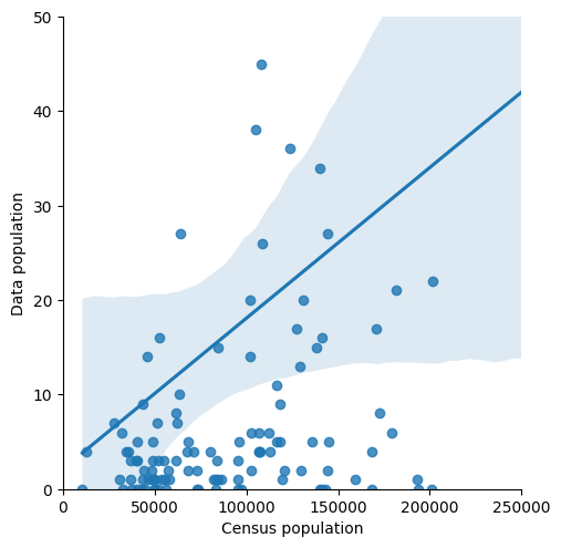
The synthetic case

We now merge our population estimate with the one given in the original shapefile in the POP column.

Results are not beautiful but remember that: - we are working on a small dataset (~200 original users) expanded to simulate many users in an arbitrary way; - the spatial tessellation may be different from the original one as we reconstructed it with a Voronoi tessellation;

While we focus on the Beijing synthetic case here, in the next section we will show the estimations for the Mexico usecase, where results are found to be in very good agreement with the empirical case.

[19]:

df_hw_locs_pd.head(4)

[19]:

	tot_pings	home_tile_ID	lat_home	lng_home	home_pings	work_tile_ID	lat_work	lng_work	work_pings
uid
82	4297.0	106.0	40.004416	116.322909	1218.0	106.0	39.997723	116.323012	1040.0
102	16531.0	106.0	39.996643	116.325115	2471.0	106.0	40.000683	116.323300	1966.0
111	11562.0	106.0	40.000315	116.322960	2240.0	106.0	40.001965	116.322623	3066.0
141	2200.0	102.0	39.981531	116.338790	78.0	89.0	39.967705	116.339616	522.0

[20]:

population_per_area = df_hw_locs_pd.reset_index().groupby("home_tile_ID").agg({
                                                "uid": "nunique",
                                                "home_pings": "sum"}).reset_index()

population_per_area = population_per_area.rename(columns={
                                                "home_tile_ID": "tile_ID",
                                                "uid": "POP_DATA",
                                                "home_pings": "pings"})
population_per_area.head(2)

[20]:

	tile_ID	POP_DATA	pings
0	0.0	6	1498.0
1	2.0	1	0.0

[21]:

# Merge with gdf
gdf_areas = pd.merge(tessellation_gdf, population_per_area, on="tile_ID", how="left")
gdf_areas["POP_DATA"] = gdf_areas["POP_DATA"].fillna(0)
gdf_areas.head(4)

[21]:

	TID	POP	M	F	AGE0	AGE15	AGE65	Address	geometry	tile_ID	POP_DATA	pings
0	257	102402	51818	50584	11322	83441	7639	北京市大兴区清源街道	POLYGON ((116.29603 39.74097, 116.31217 39.771...	0	6.0	1498.0
1	259	168444	94211	74233	17898	144834	5712	北京市大兴区黄村	POLYGON ((116.22050 39.74097, 116.22050 39.786...	1	0.0	NaN
2	262	49612	27649	21963	4472	42847	2293	北京市大兴区瀛海	POLYGON ((116.39314 39.74097, 116.39185 39.750...	2	1.0	0.0
3	92	48076	24392	23684	4975	39191	3910	北京市丰台区南苑街道	POLYGON ((116.39185 39.75000, 116.37391 39.764...	3	2.0	0.0

[22]:

sns.lmplot(x="POP", y="POP_DATA", data=gdf_areas)
# plt.loglog()
plt.xlim(0, 250000)
plt.ylim(0, 50)

plt.xlabel("Census population")
plt.ylabel("Data population")

[22]:

Text(24.625000000000007, 0.5, 'Data population')

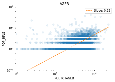
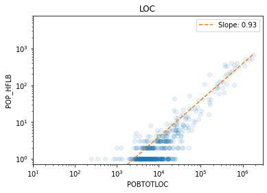
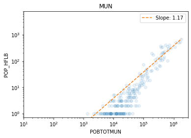
../_images/examples_mobilkit_tutorial_33_1.png

The Mexican case

We load the results of the population analysis in Mexico for the Puebla earthquake and see the agreement between census and mobility estimation at different aggregation levels, from the smallest (AGEB, street blocks) to the largest (Municipios, city level).

Note that these data are not included in the repository to preserve users’ privacy.

This section is inserted as an example to show the capabilities of the mobility data to measure the population spatial density.

[24]:

# Table-preview not shown so as not to disclose original dataset statistics
population_mexico_df = pd.read_csv("../../data/population_estimate_mexico.csv")
population_mexico_df.head(2)

[25]:

# The smallest aggregations (street block level)
mobilkit.viz.plot_pop(population_mexico_df, "AGEB")
plt.xlim(1e2, 3e4)
plt.ylim(1e-1, 1e2)

                            OLS Regression Results
==============================================================================
Dep. Variable:                      y   R-squared:                       0.075
Model:                            OLS   Adj. R-squared:                  0.074
Method:                 Least Squares   F-statistic:                     352.2
Date:                Wed, 02 Jun 2021   Prob (F-statistic):           1.25e-75
Time:                        08:16:16   Log-Likelihood:                -208.40
No. Observations:                4369   AIC:                             420.8
Df Residuals:                    4367   BIC:                             433.6
Df Model:                           1
Covariance Type:            nonrobust
==============================================================================
                 coef    std err          t      P>|t|      [0.025      0.975]
------------------------------------------------------------------------------
const         -0.5443      0.042    -13.058      0.000      -0.626      -0.463
x1             0.2211      0.012     18.766      0.000       0.198       0.244
==============================================================================
Omnibus:                      454.477   Durbin-Watson:                   1.779
Prob(Omnibus):                  0.000   Jarque-Bera (JB):              610.535
Skew:                           0.857   Prob(JB):                    2.65e-133
Kurtosis:                       3.645   Cond. No.                         41.4
==============================================================================

Notes:
[1] Standard Errors assume that the covariance matrix of the errors is correctly specified.

[25]:

(0.1, 100.0)

../_images/examples_mobilkit_tutorial_36_2.png

[26]:

# Aggregate to locality (districts) and municipio (city)
population_mexico_df["CVEGEO_LOC"] = population_mexico_df["CVEGEO"].apply(lambda s: s[:-4])
population_mexico_df["CVEGEO_MUN"] = population_mexico_df["CVEGEO_LOC"].apply(lambda s: s[:-4])

urban_areas_loc_gdf = population_mexico_df.groupby("CVEGEO_LOC").agg({
        "POP_HFLB": "sum",
        "POBTOT": "sum",
        "CVEGEO_MUN": "first",
        "CVE_LOC": "first",
        "CVE_ENT": "first",
        "CVE_MUN": "first",
    }).reset_index()

urban_areas_mun_gdf = population_mexico_df.groupby("CVEGEO_MUN").agg({
        "POP_HFLB": "sum",
        "POBTOT": "sum",
        "CVE_ENT": "first",
        "CVE_MUN": "first",
    }).reset_index()

[27]:

# The locality aggregation level (district level)
mobilkit.viz.plot_pop(urban_areas_loc_gdf, "LOC")
plt.xlim(1e1,3e6)
plt.ylim(7e-1,8e3)

                            OLS Regression Results
==============================================================================
Dep. Variable:                      y   R-squared:                       0.766
Model:                            OLS   Adj. R-squared:                  0.766
Method:                 Least Squares   F-statistic:                     1535.
Date:                Wed, 02 Jun 2021   Prob (F-statistic):          7.01e-150
Time:                        08:16:24   Log-Likelihood:                -113.13
No. Observations:                 470   AIC:                             230.3
Df Residuals:                     468   BIC:                             238.6
Df Model:                           1
Covariance Type:            nonrobust
==============================================================================
                 coef    std err          t      P>|t|      [0.025      0.975]
------------------------------------------------------------------------------
const         -3.3410      0.098    -34.198      0.000      -3.533      -3.149
x1             0.9302      0.024     39.185      0.000       0.884       0.977
==============================================================================
Omnibus:                        8.056   Durbin-Watson:                   1.578
Prob(Omnibus):                  0.018   Jarque-Bera (JB):                8.871
Skew:                           0.229   Prob(JB):                       0.0118
Kurtosis:                       3.492   Cond. No.                         29.9
==============================================================================

Notes:
[1] Standard Errors assume that the covariance matrix of the errors is correctly specified.

[27]:

(0.7, 8000.0)

../_images/examples_mobilkit_tutorial_38_2.png

[ ]:

# The municipality aggregation level
mobilkit.viz.plot_pop(urban_areas_mun_gdf, "MUN")
plt.xlim(1e1,3e6)
plt.ylim(7e-1,8e3)

                            OLS Regression Results
==============================================================================
Dep. Variable:                      y   R-squared:                       0.854
Model:                            OLS   Adj. R-squared:                  0.853
Method:                 Least Squares   F-statistic:                     1214.
Date:                Wed, 02 Jun 2021   Prob (F-statistic):           8.83e-89
Time:                        08:16:25   Log-Likelihood:                -52.923
No. Observations:                 210   AIC:                             109.8
Df Residuals:                     208   BIC:                             116.5
Df Model:                           1
Covariance Type:            nonrobust
==============================================================================
                 coef    std err          t      P>|t|      [0.025      0.975]
------------------------------------------------------------------------------
const         -4.5717      0.156    -29.313      0.000      -4.879      -4.264
x1             1.1737      0.034     34.846      0.000       1.107       1.240
==============================================================================
Omnibus:                        1.063   Durbin-Watson:                   1.894
Prob(Omnibus):                  0.588   Jarque-Bera (JB):                0.891
Skew:                          -0.158   Prob(JB):                        0.640
Kurtosis:                       3.048   Cond. No.                         35.0
==============================================================================

Notes:
[1] Standard Errors assume that the covariance matrix of the errors is correctly specified.

(0.7, 8000.0)

../_images/examples_mobilkit_tutorial_39_2.png

[ ]:

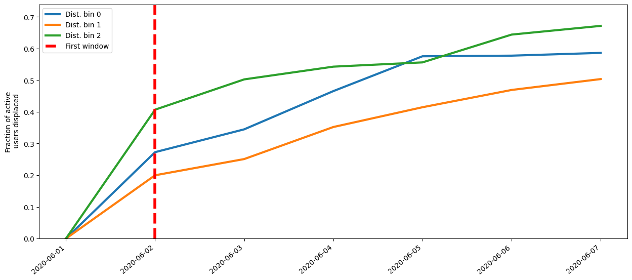
Displacement measures

Now we show how to measure the location of users in time.

We have to tell how many initial days to use to determine the original home location.

Then, we tell how many days to use for each window to determine the dynamical home location of each user (and how many pings we want at least for a night to be valid).

[28]:

# The parameters of the home location in window function
initial_days_home = 2
home_days_window = 2
start_date=None

# Compute running home location
running_home_df = mobilkit.temporal.homeLocationWindow(dd_week_hw,
                    initial_days_home=initial_days_home,
                    home_days_window=home_days_window,
                    start_date=None, stop_date=None)

Got the delta days distributed as: count    29331.000000
mean         3.639324
std          2.024058
min          0.000000
25%          2.000000
50%          4.000000
75%          5.000000
max          7.000000
Name: deltaDay, dtype: float64
Doing window 01 / 02
Doing window 02 / 02

[29]:

# We now have for ech user and time window (with its initial date) the location
# where he supposedly spent the night and how many pings are recorded there
running_home_df.head(4)

[29]:

	pings	tile_ID	uid	window_date
0	9	106	1	2020-06-01 00:00:00+00:00
1	273	106	2	2020-06-01 00:00:00+00:00
2	314	106	4	2020-06-01 00:00:00+00:00
3	212	106	7	2020-06-01 00:00:00+00:00

After we determined the residing area for each user/night we use mobilkit.temporal.computeDisplacementFigures to get four objects containing the results of the analysis.

The ones we are interested in are: - pivoted_df telling for each night where a user slept; - count_users_per_area telling for each area how many users originally residing there were active and how many were displaced on that day;

[30]:

# Compute displacement figures

minimum_pings_per_night = 3

pivoted_df, original_home,\
    heaps, count_users_per_area = mobilkit.temporal.computeDisplacementFigures(
        running_home_df, minimum_pings_per_night=minimum_pings_per_night,
)

# The lat lon of the center
epicenter = [tessellation_gdf.unary_union.centroid.xy[1][0],
             tessellation_gdf.unary_union.centroid.xy[0][0]]

# Assess displacement based on distance from epicenter
fig, gdf_enriched = mobilkit.temporal.plotDisplacement(count_users_per_area, pivoted_df,
                                   tessellation_gdf,
                                   epicenter=epicenter,
                                   bins=3)

../_images/examples_mobilkit_tutorial_45_0.png

[31]:

# Viusualize the distance bins
fig, ax = plt.subplots(1,1,figsize=(12,12))
ax.set_aspect("equal")
gdf_enriched.plot("distance_bin", legend=True, ax=ax)

[31]:

<Axes: >

../_images/examples_mobilkit_tutorial_46_1.png

[32]:

# Visualize the displacement rate per area on a given date
dates_sorted = sorted(pivoted_df.columns)
selected_date_index = 2

gdf_enriched["displaced_at_date"] = gdf_enriched["tile_ID"].apply(lambda a:
                                                      count_users_per_area[a]["displaced"][selected_date_index]
                                                      / max(1, count_users_per_area[a]["active"][selected_date_index])
                                                      if a in count_users_per_area else None)

fig, ax = plt.subplots(1,1,figsize=(15,12))
ax.set_aspect("equal")
gdf_enriched.plot("displaced_at_date", legend=True, ax=ax, legend_kwds={'label': "Displaced fraction"})
plt.title("Date = %s" % dates_sorted[selected_date_index].strftime("%d/%m/%Y"))

[32]:

Text(0.5, 1.0, 'Date = 03/06/2020')

../_images/examples_mobilkit_tutorial_47_1.png

Land use

For this particular analysis we use the daily data because they map to more users (more stats).

We start assigning every ping to a location and then we compute the activity profiles.

[33]:

dd_usr_with_zones, tessellation_gdf = mobilkit.spatial.tessellate(dd_users_raw,
                                                                  tesselation_shp=voronoi_file,
                                                                  filterAreas=True)
dd_usr_with_zones.head()

[33]:

	UTC	acc	datetime	lat	lng	tile_ID
0	1591008784	1	2020-06-01 10:53:04+00:00	39.984702	116.318417	99
1	1591008790	1	2020-06-01 10:53:10+00:00	39.984683	116.318450	99
2	1591008795	1	2020-06-01 10:53:15+00:00	39.984686	116.318417	99
3	1591008800	1	2020-06-01 10:53:20+00:00	39.984688	116.318385	99
4	1591008805	1	2020-06-01 10:53:25+00:00	39.984655	116.318263	99

[34]:

# This is the time period over which we want to compute the average activity of an area
# normalization="total" tells to the program to normalize the activity of each area dividing it by
# the overall volume of pings or users found in all the ROI. See the docs for other normalization
# strategies.
selected_profile_period = "day"
total_profiles_df = mobilkit.temporal.computeTemporalProfile(dd_usr_with_zones, timeBin="H",
                                                             byArea=True,
                                                             profile=selected_profile_period,
                                                            normalization="total").compute()

[35]:

# We compute the residual activity of users found in a given area
signal_column = "users"
results, mappings =  mobilkit.temporal.computeResiduals(total_profiles_df,
            signal_column=signal_column, profile=selected_profile_period)

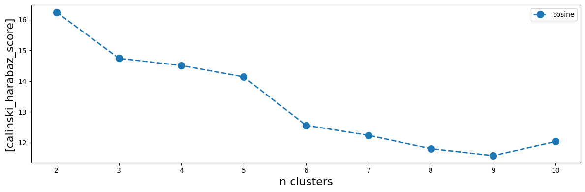
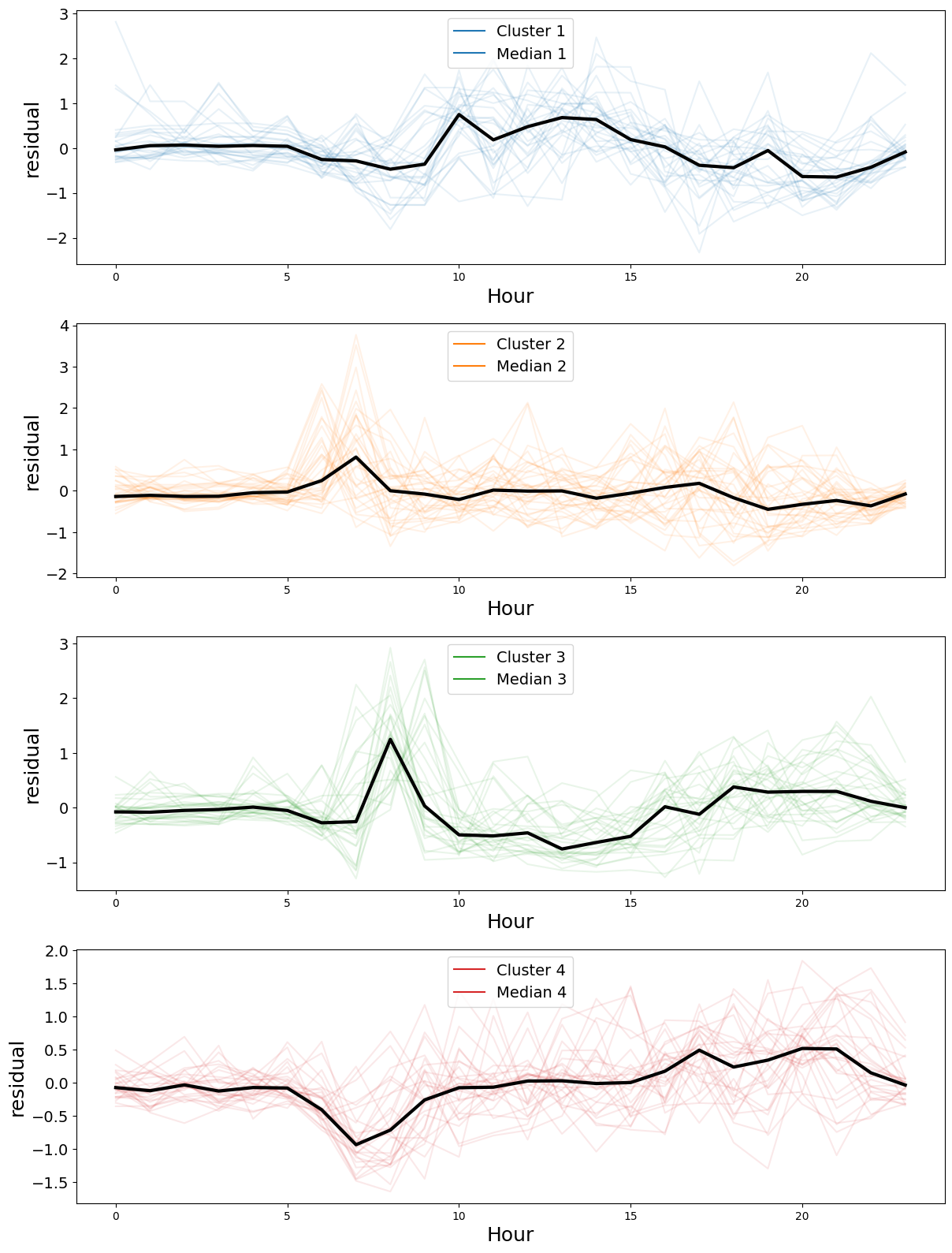
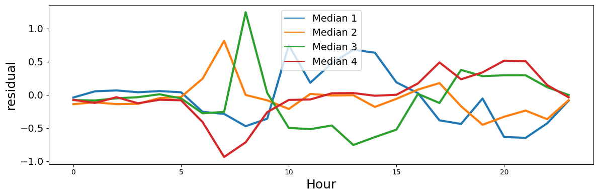
Finally we try to cluster these profiles in some groups. We use hierarchical clustering of the residual activity profiles using the cosine metric.

This plot tells us the score of the partitioning, the higer the better.

Given that we do not have many data we select n=4 clusters even though we do not have a clear maximum.

[36]:

signal_to_use = "residual"
metric = "cosine"  # The metric to be used in computing the distance matrix
results_clusters = mobilkit.tools.computeClusters(results,
                                                  signal_to_use,
                                                  metric=metric,
                                                  nClusters=range(2,11))

# Visualize score
ax_score = mobilkit.tools.checkScore(results_clusters)

Done n clusters = 02
Done n clusters = 03
Done n clusters = 04
Done n clusters = 05
Done n clusters = 06
Done n clusters = 07
Done n clusters = 08
Done n clusters = 09
Done n clusters = 10

../_images/examples_mobilkit_tutorial_53_1.png

[37]:

# Plot clusters profiles and map: We select 4 clusters and plot their profiles and map.
nClusters = 4
ax = mobilkit.tools.visualizeClustersProfiles(results_clusters,
            nClusts=nClusters, showMean=False, showMedian=True, showCurves=True)

../_images/examples_mobilkit_tutorial_54_0.png

[38]:

# We compare all the medians activity profiles of the 4 clusters
ax = mobilkit.tools.visualizeClustersProfiles(results_clusters,
            nClusts=nClusters, showMean=False, showMedian=True, showCurves=False, together=True)

../_images/examples_mobilkit_tutorial_55_0.png

[39]:

# We plot the map of the clusters, with the same colors as before.
gdf_update, ax_mappa = mobilkit.tools.plotClustersMap(tessellation_gdf, results_clusters,
                                                      mappings, nClusts=nClusters)

../_images/examples_mobilkit_tutorial_56_0.png

[ ]: