Mobility for resilience: population analysis
This notebook shows the preliminary steps done using mobilkit to load raw HFLB data, determine the population estimates of each area and prepare the data for displacement and POI visit rates.
We start loading raw HFLB data using the mobilkit.loader module.
[1]:
%matplotlib inline
%config Completer.use_jedi = False

import os
import sys
from copy import copy, deepcopy
from glob import glob
from collections import Counter
import pytz
from datetime import datetime

import matplotlib.pyplot as plt
from matplotlib.gridspec import GridSpec
from mpl_toolkits.axes_grid1 import make_axes_locatable
from pandas.plotting import register_matplotlib_converters
register_matplotlib_converters()

import numpy as np
import pandas as pd
import seaborn as sns
import geopandas as gpd
import contextily as ctx
import pyproj
from scipy import stats
from sklearn import cluster

import dask
from dask.distributed import Client
from dask import dataframe as dd

### import mobility libraries
import skmob
import mobilkit

sns.set_context("notebook", font_scale=1.5)
[10]:
dask.__version__ ### tested using Dask version 2020.12.0
[10]:
'2020.12.0'
Load data
Set up Dask
Notes:
Use Dask library for high-speed computation on edge computer
accumulates tasks and runs actual computation when “.compute()” is given
If cluster computing is available, using PySpark is recommended
Click the URL of the Dashboard below to monitor progress
[12]:
client = Client(address="127.0.0.1:8786") ### choose number of cores to use
client
[12]:
Client
|
Cluster
|
Load raw data using mobilkit interface
[16]:
datapath = "../../data/"
outpath  = "../../results/"

### define temporal cropping parameters (including these dates)
timezone = "America/Mexico_City"

startdate = "2017-09-04"
enddate   = "2017-10-08"

nightendtime = "09:00:00"
nightstarttime = "18:00:00"

# How to translate the original columns in the mobilkit's nomenclature
colnames = {"id": "uid",
            "gaid": "gaid",
            "hw": "hw",
            "lat": "lat",
            "lon": "lng",
            "accuracy": "acc",
            "unixtime": "UTC",
            "noise": "noise"
           }

# Wehere raw data are stored
filepath = "/data/DataWB/sample/*.part"
ddf = mobilkit.loader.load_raw_files(filepath,
                                     version="wb",
                                     sep=",",
                                     file_schema=colnames,
                                     start_date=startdate,
                                     stop_date=enddate,
                                     timezone=timezone,
                                     header=True,
                                     minAcc=300.,
                                    )
Quickly compute min/max of space-time
Use the mobilkit and skmob column names notations.
[23]:
dmin, dmax, lonmin, lonmax, latmin, latmax = dask.compute(ddf.UTC.min(),
                                                          ddf.UTC.max(),
                                                          ddf.lng.min(), ddf.lng.max(),
                                                          ddf.lat.min(), ddf.lat.max()
                                                         )
[54]:
print(mobilkit.loader.fromunix2fulldate(dmin),
      mobilkit.loader.fromunix2fulldate(dmax))
print(lonmin, lonmax, latmin, latmax)
2017-09-03 10:07:17 2017-10-09 07:13:57
-105 -95 15.5 22.55
[55]:
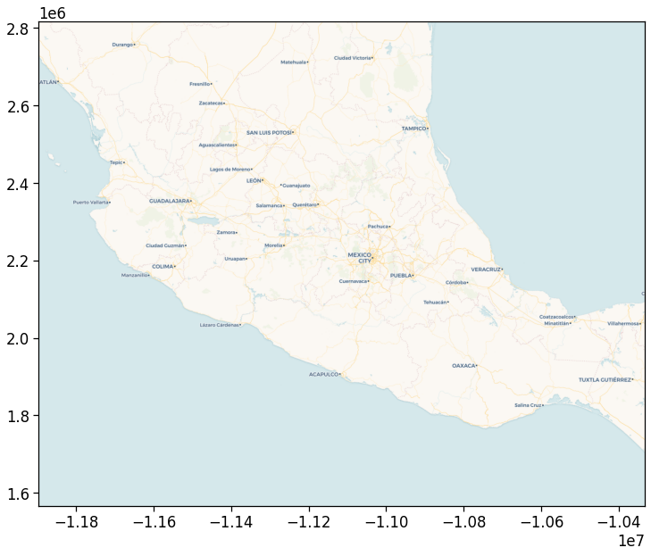
boundary = (lonmin, latmin, lonmax, latmax)
[55]:
(-105, 15.5, -95, 22.55)
[57]:
mobilkit.viz.visualize_boundarymap(boundary)
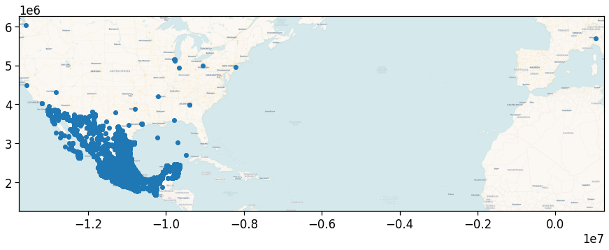
Sample of dataset (choose a very small fraction)
[28]:
%%time
ddf_sample = ddf.sample(frac=0.0001).compute()
CPU times: user 11.9 s, sys: 736 ms, total: 12.6 s
Wall time: 5min 11s
[29]:
len(ddf_sample)
[29]:
32750
[30]:
mobilkit.viz.visualize_simpleplot(ddf_sample)
/home/ubi/Sandbox/mobilkit_dask/mobenv/lib/python3.9/site-packages/pyproj/crs/crs.py:53: FutureWarning: '+init=<authority>:<code>' syntax is deprecated. '<authority>:<code>' is the preferred initialization method. When making the change, be mindful of axis order changes: https://pyproj4.github.io/pyproj/stable/gotchas.html#axis-order-changes-in-proj-6
  return _prepare_from_string(" ".join(pjargs))
Clean data
Some ideas on data cleaning:
geographical boundary; analyze data only within a specific area
temporal boundary; analyze data only within a specific timeframe
Users’ data quality; select users with more than X datapoints, etc.
Geographical boundary
[31]:
### define boundary box: (min long, min lat, max long, max lat)
# ==== Parameters === #
bbox = (-106.3, 15.5, -86.3, 29.1)
[32]:
# ddf_sc = ddf.map_partitions(data_preprocess.crop_spatial, bbox)
ddf_sc = ddf.map_partitions(mobilkit.loader.crop_spatial, bbox)
Temporal boundary
These computation gets done automatically when loading now.
We only have to filter night hours.
[34]:
nightendtime = "09:00:00"
nightstarttime = "18:00:00"

ddf_tc2 = ddf_sc.map_partitions(mobilkit.loader.crop_time,
                                nightendtime,
                                nightstarttime,
                                timezone)
select users with sufficient data points
users_totalXpoints : select users with more than X data points throughout entire period
users_Xdays : select users with observations of more than X days
users_Xavgps : select users with more than X observations per day
users_Xdays_Xavgps : select users that satisfy both criteria
[38]:
# ==== Parameters === #
mindays = 3
avgpoints = 1

ddf = ddf.assign(uid=ddf["id"])
users_stats = mobilkit.stats.userStats(ddf).compute()
valid_users = set(users_stats[
                (users_stats["avg"] > avgpoints)
                & (users_stats["daysActive"] > mindays)
                ]["uid"].values)

ddf_clean = mobilkit.stats.filterUsersFromSet(ddf, valid_users)
# I do not have this col...
# ddf_clean_homework = ddf_clean[ddf_clean["hw"]=="HOMEWORK"]
# I keep only events during night
ddf_clean_homework = ddf_clean_homework[~ddf_clean_homework["datetime"].dt.hour.between(8,19)]
Home location estimation
Estimation using Meanshift
took ~ 2 hours 15 minutes for entire dataset (mindays=1, avgpoints=0.1)
We compute home location and we later split it into its latitude and longitude.
[42]:
id_home = ddf_clean_homework.groupby("uid").apply(mobilkit.spatial.meanshift)\
                                .compute()\
                                .reset_index()\
                                .rename(columns={0:"home"})
toc = datetime.now()
print("Number of IDs with estimated homes: ",len(id_home))
<ipython-input-42-2437fa6c87f0>:2: UserWarning: `meta` is not specified, inferred from partial data. Please provide `meta` if the result is unexpected.
  Before: .apply(func)
  After:  .apply(func, meta={'x': 'f8', 'y': 'f8'}) for dataframe result
  or:     .apply(func, meta=('x', 'f8'))            for series result
  id_home = ddf_clean_homework.groupby("uid").apply(mobilkit.spatial.meanshift)\
/home/ubi/Sandbox/mobilkit_dask/mobenv/lib/python3.9/site-packages/distributed/worker.py:3445: UserWarning: Large object of size 19.15 MB detected in task graph:
  (['a81dbcb8f4c35834d6619a45d67f34d95911fab1318710d ... e5ce12ca182'],)
Consider scattering large objects ahead of time
with client.scatter to reduce scheduler burden and
keep data on workers

    future = client.submit(func, big_data)    # bad

    big_future = client.scatter(big_data)     # good
    future = client.submit(func, big_future)  # good
  warnings.warn(
Number of IDs with estimated homes: 279541
[44]:
### save to csv file
id_home.to_csv("../data/"+"id_home_"+str(mindays)+"_"+str(avgpoints).replace(".","")+".csv")
[46]:
id_home["lon"] = id_home["home"].apply(lambda x : x[0])
id_home["lat"] = id_home["home"].apply(lambda x : x[1])
id_home = id_home.drop(columns=["home"])[["uid","lon","lat"]]
id_home.lon = id_home.lon.astype("float64")
id_home.lat = id_home.lat.astype("float64")
[48]:
# Create a geodataframe for spatial queries
idhome_gdf = gpd.GeoDataFrame(id_home, geometry=gpd.points_from_xy(id_home.lon, id_home.lat))
Compute administrative region for each ID
manzana shape data (for only urban areas)
[49]:
### load shape data
areas = ["09_Manzanas_INV2016_shp","17_Manzanas_INV2016_shp",
         "21_Manzanas_INV2016_shp","29_Manzanas_INV2016_shp"]
manz_shp = gpd.GeoDataFrame()
for i,a in enumerate(areas):
    manz_f = "data/spatial/manzanas_shapefiles/"+a+"/"
    manz_shp1 = gpd.read_file(manz_f)
    manz_shp = manz_shp.append(manz_shp1, ignore_index=True)
    print("done",i)
done 0
done 1
done 2
done 3
[50]:
manz_shp = manz_shp[["geometry","CVEGEO",'ENT','MUN','LOC','AGEB', 'MZA']]
manz_shp.head()
[50]:
| geometry | CVEGEO | ENT | MUN | LOC | AGEB | MZA | |
|---|---|---|---|---|---|---|---|
| 0 | POLYGON ((-99.20644 19.51393, -99.20640 19.513... | 0900200010010001 | 09 | 002 | 0001 | 0010 | 001 |
| 1 | POLYGON ((-99.20594 19.51418, -99.20586 19.514... | 0900200010010002 | 09 | 002 | 0001 | 0010 | 002 |
| 2 | POLYGON ((-99.20526 19.51279, -99.20526 19.512... | 0900200010010003 | 09 | 002 | 0001 | 0010 | 003 |
| 3 | POLYGON ((-99.20563 19.51279, -99.20562 19.512... | 0900200010010004 | 09 | 002 | 0001 | 0010 | 004 |
| 4 | POLYGON ((-99.20655 19.51278, -99.20653 19.512... | 0900200010010005 | 09 | 002 | 0001 | 0010 | 005 |
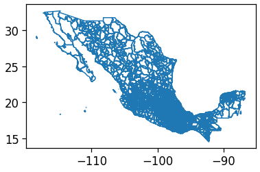
By Entidad or Municipio stratification
[51]:
adm2_f = datapath+"spatial/boundaries_shapefiles/mex_admbnda_adm2_govmex/"
adm2_shp = gpd.read_file(adm2_f)
adm2_shp.boundary.plot()
[51]:
<AxesSubplot:>
[52]:
adm2_shp = adm2_shp[["ADM2_PCODE","geometry"]]
adm2_shp["ent"] = adm2_shp["ADM2_PCODE"].apply(lambda x : x[2:4])
adm2_shp["entmun"] = adm2_shp["ADM2_PCODE"].apply(lambda x : x[2:])
[53]:
adm2_shp.head()
[53]:
| ADM2_PCODE | geometry | ent | entmun | |
|---|---|---|---|---|
| 0 | MX01001 | POLYGON ((-102.09775 22.02325, -102.09857 22.0... | 01 | 01001 |
| 1 | MX01002 | POLYGON ((-101.99941 22.21951, -101.99940 22.2... | 01 | 01002 |
| 2 | MX01003 | POLYGON ((-102.57625 21.96778, -102.57626 21.9... | 01 | 01003 |
| 3 | MX01004 | POLYGON ((-102.25320 22.37449, -102.25239 22.3... | 01 | 01004 |
| 4 | MX01005 | POLYGON ((-102.31034 22.03716, -102.30653 22.0... | 01 | 01005 |
Spatial join with manzana data
compute what geographical boundar each home location is in
[2]:
id_manz = gpd.sjoin(idhome_gdf, manz_shp, how="inner", op='within')
id_manz["loc_code"]  = id_manz["CVEGEO"].apply(lambda x : x[:9])
id_manz["ageb_code"] = id_manz["CVEGEO"].apply(lambda x : x[:13])
id_manz["mza_code"]  = id_manz["CVEGEO"].apply(lambda x : x[:16])
id_manz = id_manz.drop(columns=["LOC","AGEB","MZA"])
Spatial join with entidad/muncipio data
[3]:
id_entmun = gpd.sjoin(idhome_gdf, adm2_shp, how="inner", op='within')
Validation using census population data
Population data for all levels
[56]:
poppath = datapath+"sociodemographic/populationdata/"
df_pop = pd.DataFrame()
for es in ["09","17","21","29"]:
    pop = poppath+"resultados_ageb_urbana_"+es+"_cpv2010.csv"
    df_pop1 = pd.read_csv(pop)[["entidad","mun","loc","ageb","mza","pobtot"]]
    df_pop = df_pop.append(df_pop1, ignore_index=True)

df_pop["CVEGEO"] = df_pop.apply(lambda row: str(row["entidad"]).zfill(2)+
                                str(row["mun"]).zfill(3)+
                                str(row["loc"]).zfill(4)+
                                str(row["ageb"]).zfill(4)+
                                str(row["mza"]).zfill(3), axis=1)
[57]:
df_pop.head()
[57]:
| entidad | mun | loc | ageb | mza | pobtot | CVEGEO | |
|---|---|---|---|---|---|---|---|
| 0 | 9 | 0 | 0 | 0000 | 0 | 8851080 | 0900000000000000 |
| 1 | 9 | 2 | 0 | 0000 | 0 | 414711 | 0900200000000000 |
| 2 | 9 | 2 | 1 | 0000 | 0 | 414711 | 0900200010000000 |
| 3 | 9 | 2 | 1 | 0010 | 0 | 3424 | 0900200010010000 |
| 4 | 9 | 2 | 1 | 0010 | 1 | 202 | 0900200010010001 |
Entidad level
[59]:
ent_ids = id_entmun.groupby("ent").uid.count().reset_index()
ent_pop = df_pop[(df_pop["mun"]==0) & (df_pop["loc"]==0)
                 & (df_pop["ageb"]=="0000") & (df_pop["mza"]==0)][["entidad","pobtot"]]
ent_pop["ent"] = ent_pop["entidad"].apply(lambda x : str(x).zfill(2))
ent_ids_pop = ent_pop.merge(ent_ids, on="ent")
Municipio level
[60]:
mun_ids = id_entmun.groupby("entmun").uid.count().reset_index()
mun_pop = df_pop[(df_pop["mun"]!=0) & (df_pop["loc"]==0)
                 & (df_pop["ageb"]=="0000") & (df_pop["mza"]==0)][["CVEGEO","pobtot"]]
mun_pop["entmun"] = mun_pop["CVEGEO"].apply(lambda x : str(x)[:5])
mun_ids_pop = mun_pop.merge(mun_ids, on="entmun")
Localidades level
[61]:
loc_ids = id_manz.groupby("loc_code").uid.count().reset_index()
loc_pop = df_pop[(df_pop["mun"]!=0) & (df_pop["loc"]!=0)
                 & (df_pop["ageb"]=="0000") & (df_pop["mza"]==0)][["CVEGEO","pobtot"]]
loc_pop["loc_code"] = loc_pop["CVEGEO"].apply(lambda x : str(x)[:9])
loc_ids_pop = loc_pop.merge(loc_ids, on="loc_code")
AGEB level
[62]:
ageb_ids = id_manz.groupby("ageb_code").uid.count().reset_index()
ageb_pop = df_pop[(df_pop["mun"]!=0) & (df_pop["loc"]!=0)
                 & (df_pop["ageb"]!="0000") & (df_pop["mza"]==0)][["CVEGEO","pobtot"]]
ageb_pop["ageb_code"] = ageb_pop["CVEGEO"].apply(lambda x : str(x)[:13])
ageb_ids_pop = ageb_pop.merge(ageb_ids, on="ageb_code")
Manzana level
[63]:
mza_ids = id_manz.groupby("mza_code").uid.count().reset_index()
mza_pop = df_pop[(df_pop["mun"]!=0) & (df_pop["loc"]!=0)
                 & (df_pop["ageb"]!="0000") & (df_pop["mza"]!=0)][["CVEGEO","pobtot"]]
mza_pop["mza_code"] = mza_pop["CVEGEO"].apply(lambda x : str(x)[:17])
mza_ids_pop = mza_pop.merge(mza_ids, on="mza_code")
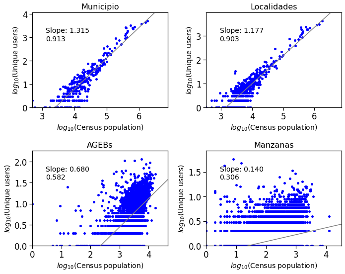
Plot census population vs MP data
[64]:
def plot_compare(df, ax, title):
    df["logpop"] = np.log10(df["pobtot"])
    df["loguser"] = np.log10(df["uid"])
    df = df.replace([np.inf, -np.inf], np.nan).dropna()
#     for col in set(df["color"].values):
#         df_thiscol = df[df["color"]==col]
    ax.scatter(df["logpop"].values, df["loguser"].values, color="b", s=15)
    c1, i1, s1, p_value, std_err = stats.linregress(df["logpop"].values, df["loguser"].values)
    ax.plot([0,np.max(df["logpop"])*1.1],[i1,i1+np.max(df["logpop"])*1.1*c1],
            linestyle="-", color="gray")
    ax.set_xlim(np.min(df["logpop"]),np.max(df["logpop"])*1.1)
    ax.set_ylim(0,np.max(df["loguser"])*1.1)
    ax.set_xlabel(r"$log_{10}$(Census population)", fontsize=14)
    ax.set_ylabel(r"$log_{10}$(Unique users)", fontsize=14)
    ax.annotate("Slope: "+str(c1)[:5]+"\n"+str(s1)[:5], #+utils.stars(p_value),
                        xy=(.1,0.7),
                        xycoords='axes fraction', color="k", fontsize=14)
    ax.set_title(title, fontsize=16)
[65]:
fig = plt.figure(figsize=(10,8))
gs=GridSpec(2,2)

ax0 = fig.add_subplot(gs[0,0])
plot_compare(mun_ids_pop, ax0, "Municipio")

ax1 = fig.add_subplot(gs[0,1])
plot_compare(loc_ids_pop, ax1, "Localidades")

ax2 = fig.add_subplot(gs[1,0])
plot_compare(ageb_ids_pop, ax2, "AGEBs")

ax3 = fig.add_subplot(gs[1,1])
plot_compare(mza_ids_pop, ax3, "Manzanas")

plt.tight_layout()
# plt.savefig(outpath+"represent_manzana_eq.png",
#             dpi=300, bbox_inches='tight', pad_inches=0.05)
plt.show()
/home/ubi/Sandbox/mobilkit_dask/mobenv/lib/python3.9/site-packages/pandas/core/arraylike.py:274: RuntimeWarning: divide by zero encountered in log10
  result = getattr(ufunc, method)(*inputs, **kwargs)
/home/ubi/Sandbox/mobilkit_dask/mobenv/lib/python3.9/site-packages/pandas/core/arraylike.py:274: RuntimeWarning: divide by zero encountered in log10
  result = getattr(ufunc, method)(*inputs, **kwargs)
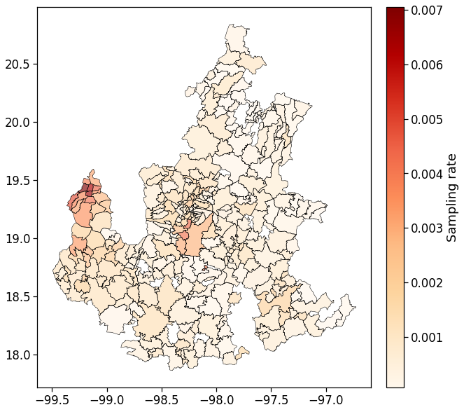
Plot population on map
[66]:
mun_ids_pop["rate"] = mun_ids_pop["uid"]/mun_ids_pop["pobtot"]
mun_ids_pop["pcode"] = mun_ids_pop["entmun"].apply(lambda x : "MX"+str(x))

mun_ids_pop_shp = adm2_shp.merge(mun_ids_pop, on="entmun", how="right")
[68]:
fig,ax = plt.subplots(figsize=(10,10))
divider = make_axes_locatable(ax)
cax = divider.append_axes("right", size="5%", pad=0.1)
mun_ids_pop_shp.plot(ax=ax, column='rate', cmap='OrRd', legend=True,
                    cax=cax, legend_kwds={'label': "Sampling rate"}, alpha=0.65)
mun_ids_pop_shp.boundary.plot(ax=ax, color="k", linewidth=0.5)
[68]:
<AxesSubplot:>
[ ]: